In modern actuarial science, there is an inherent tension between predictive accuracy and model transparency. While ensemble tree-based models like Gradient Boosting Machines (GBMs) frequently outperform traditional Generalized Linear Models (GLMs), their “black-box” nature presents significant hurdles for model governance, regulatory compliance, and price filing.
This notebook demonstrates a solution using Maximum Interpretation Decomposition (MID) via the {midr} package in R.
WarningCompatibility Notice
This article relies on features introduced in midr (>= 0.6.0). Please ensure your packages are up to date.
What is MID?
MID is a functional decomposition method that deconstructs a black-box prediction function \(f(\mathbf{X})\) into several interpretable components: an intercept \(g_\emptyset\), main effects \(g_j(X_j)\), and second-order interactions \(g_{jk}(X_j, X_k)\), minimizing the squared residuals \(\mathbf{E}\left[g_D(\mathbf{X})^2\right]\):
To ensure the uniqueness and identifiability of each component, MID imposes centering and probability-weighted minimum-norm constraints on the decomposition.
By approximating a black-box model with this surrogate structure, we can derive a representation that retains the superior predictive power of machine learning models without sacrificing actuarial transparency.
Setting Up
We begin by setting up the environment and loading the necessary libraries. We will use a standard actuarial claim dataset (freMTPL2freq in CASdatasets), split into 338,995 training and 338,996 testing observations.
Code
# data manipulationlibrary(arrow)library(dplyr)# predictive modelinglibrary(lightgbm)# surrogate modelinglibrary(midr)# visualizationlibrary(ggplot2)library(patchwork)# load training and testing datasetstrain <-read_parquet("data/train.parquet")test <-read_parquet("data/test.parquet")
A key component of our evaluation is the Weighted Mean Poisson Deviance defined as follows:
GBMs such as LightGBM often yield superior predictive power by capturing high-order interactions. However, this accuracy comes at the cost of being a black box.
We use {midr} to replicate the LightGBM model. By including interaction terms in the model formula, we allow the surrogate to capture the joint relationships that the GBM has learned. The goal is to approximate the LightGBM function \(f_{LGB}(\mathbf{x})\) with our interpretable structure \(g^*(\mathbf{x})\):
Including all second-order interactions using the (...)^2 syntax results in \(p(p-1)/2\) interaction terms. For high-dimensional data, this can be memory-intensive.
To measure how successfully our surrogate replicates the LightGBM model, we use the Uninterpreted Ratio (UR) or the R-squared score (\(R^2 = 1 - UR\)) on the link scale (\(\log\) scale).
The MID model achieves a very low uninterpreted ratio. Only 7.16% of the variance in the model predictions on the log-transformed scale is left unexplained.
Code
# evaluate fitted surrogate on testing setpred_mid_lgb =predict(mid_lgb, test, type ="response")# calculate R-squared on testing datasetR2_test <-weighted.loss(x =log(pred_fit_lgb),y =log(pred_mid_lgb),w = test$Exposure,method ="r2")UR_test <-1- R2_testR2_test_response <-weighted.loss(x = pred_fit_lgb,y = pred_mid_lgb,w = test$Exposure,method ="r2")UR_test_response <-1- R2_test_responseUR_train <- mid_lgb$ratio[1L]UR_train_response <- mid_lgb$ratio[2L]cat("Uninterpreted Ratio on the training set:\n",sprintf(" %.4f in the log-transformed scale\n %.4f in the original scale\n", UR_train, UR_train_response ),"Uninterpreted Ratio on the testing set:\n",sprintf(" %.4f in the log-transformed scale\n %.4f in the original scale", UR_test, UR_test_response ),sep ="")
Uninterpreted Ratio on the training set:
 0.0716 in the log-transformed scale
 0.1815 in the original scale
Uninterpreted Ratio on the testing set:
 0.0705 in the log-transformed scale
 0.2135 in the original scale
Feature Effects
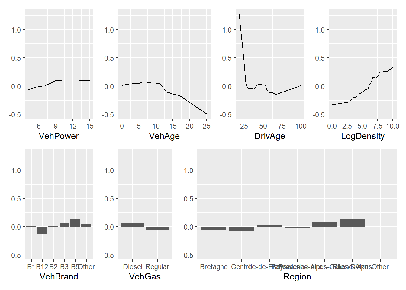
The LightGBM model can now be inspected through a transparent additive approximation. We can visualize each main effect \(g_j\) using ggplot2-based outputs via ggmid(). The model correctly identifies higher risks for young drivers (DrivAge) and highly populated areas (LogDensity).
Code
wrap_plots(lapply(mid.plots(mid_lgb), function(x) x +labs(y =NULL)),design ="AAAAABBBBBCCCCCDDDDD\nEEEEEFFFFGGGGGGGGGGG")
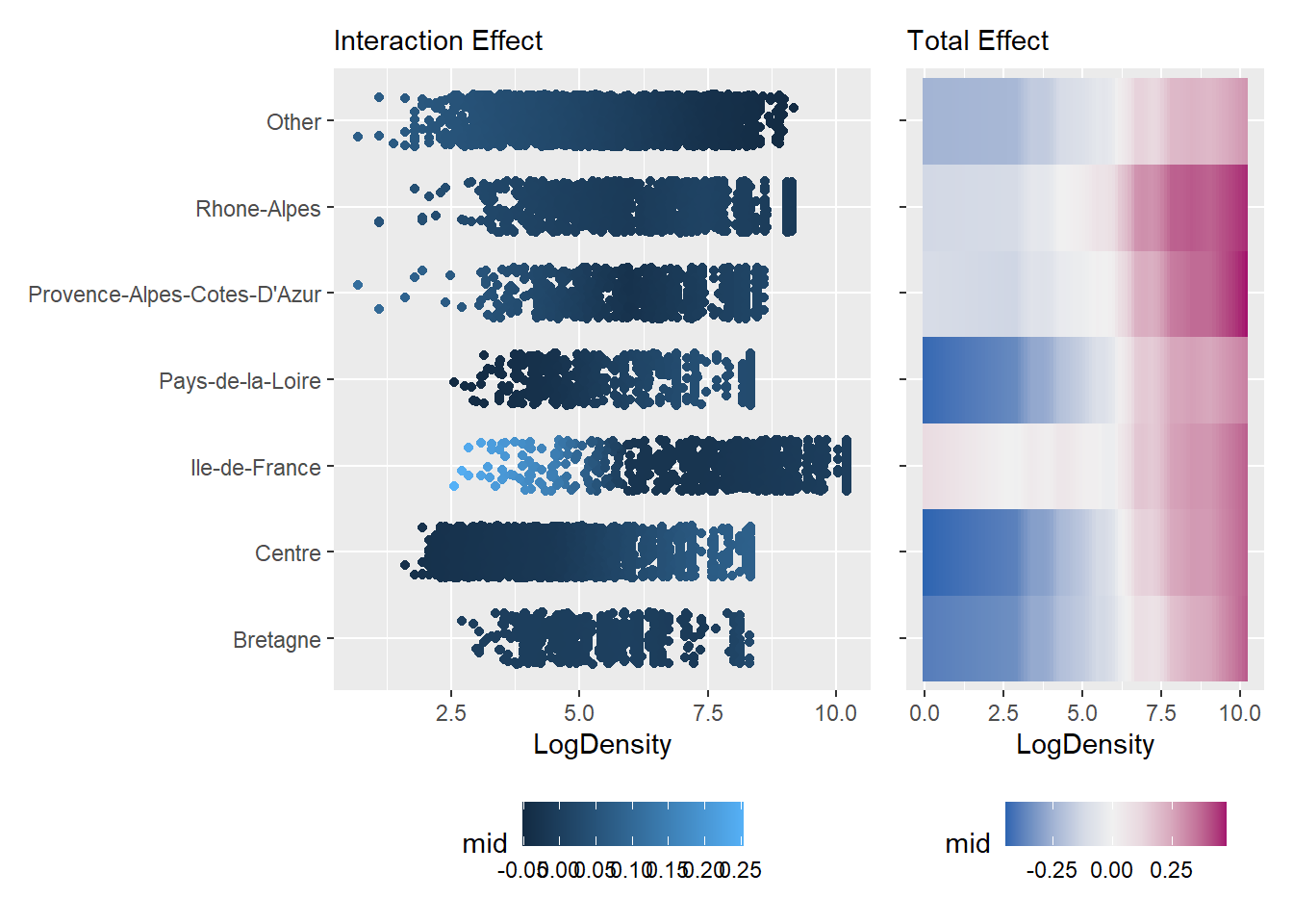
A key advantage of {midr} is its ability to isolate interaction effects \(g_{jk}\) from main effects \(g_j\). For example, while the main effect of LogDensity is generally increasing, we can learn from the interaction model that the risk remains high even in low-density areas specifically in Île-de-France.
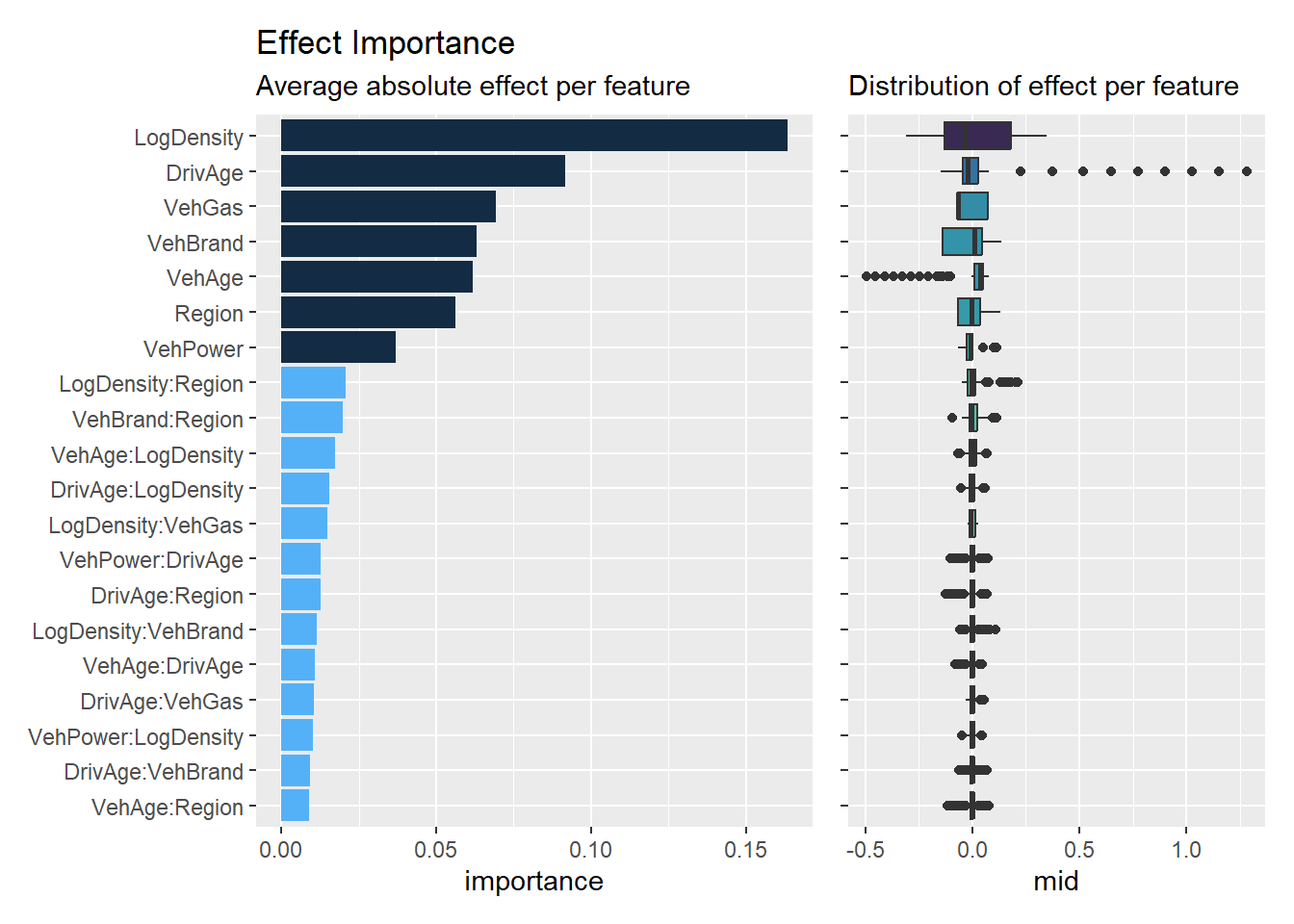
To rank the influence of each component discovered in the LightGBM model, we calculate the Effect Importance, defined as the average absolute contribution. This is highly useful to know which effects are important and non-negligible.
Code
imp_lgb <-mid.importance(mid_lgb, data = train, max.nsamples =2000)wrap_plots(nrow =1, widths =c(4, 3),ggmid(imp_lgb, theme ="bluescale@qual", max.nterms =20) +labs(title ="Effect Importance",subtitle ="Average absolute effect per feature") +theme(legend.position ="none"),ggmid(imp_lgb, type ="boxplot", theme ="mako_r", max.nterms =20) +labs(title ="",subtitle ="Distribution of effect per feature") +scale_y_discrete(labels =NULL) +theme(legend.position ="none"))
Conditional Expectation
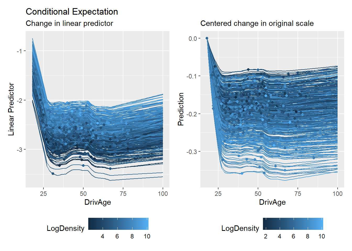
We further explore the model’s behavior using the ICE plot. In the MID framework, the variation in ICE curves for a feature \(j\) is explicitly governed by the interaction terms \(g_{jk}\) identified from the LightGBM model.
Code
ice_lgb_link <-mid.conditional(mid_lgb, type ="link", variable ="DrivAge")ice_lgb <-mid.conditional(mid_lgb, variable ="DrivAge")wrap_plots(nrow =1,ggmid(ice_lgb_link, var.color = LogDensity) +theme(legend.position ="bottom") +labs(y ="Linear Predictor",title ="Conditional Expectation",subtitle ="Change in linear predictor"),ggmid(ice_lgb, type ="centered", var.color = LogDensity) +theme(legend.position ="bottom") +labs(y ="Prediction", title ="",subtitle ="Centered change in original scale"))
Additive Attribution
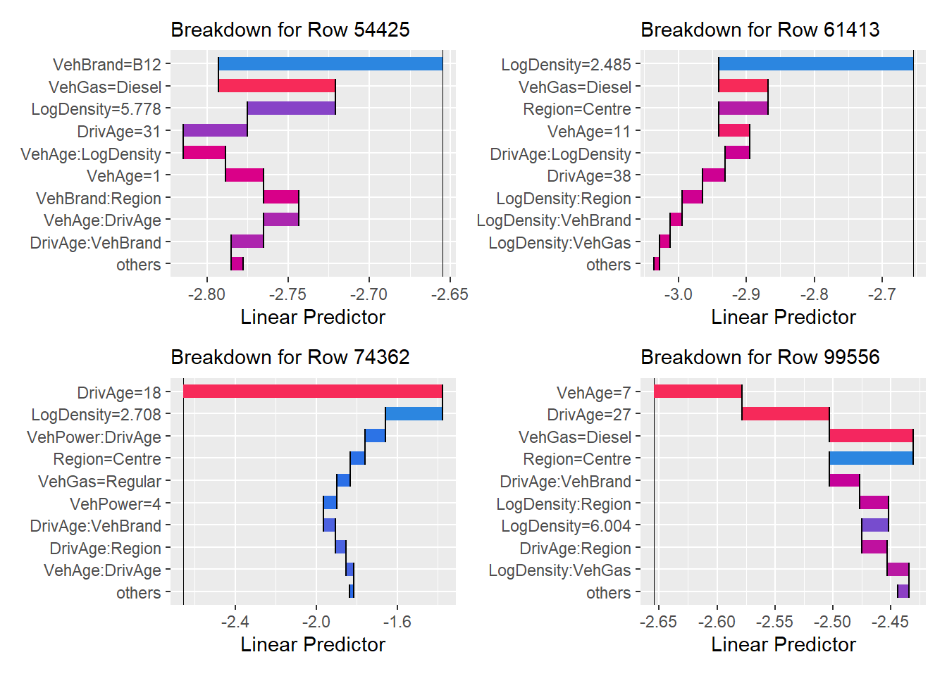
Finally, we perform an Additive Breakdown for individual predictions. This provides an exact allocation of the LightGBM’s prediction into the terms of our surrogate model, serving as a powerful tool for instance-level explanation.
While the previous examples focused on scalar predictions (e.g., expected claim frequency), the MID algorithm can be naturally extended to handle matrix-valued outputs. This extension unlocks several advanced actuarial applications without fundamentally changing the underlying algorithm:
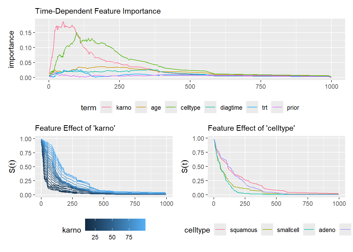
Survival Analysis (SurvMID(t))
In survival analysis, models predict survival curves \(S(t)\) evaluated at \(m\) distinct time points. By applying the matrix-extended MID, we obtain time-dependent main effects \(g_j(x_j, t)\) and interactions \(g_{jk}(x_j, x_k, t)\). This allows actuaries to visualize how a specific risk factor’s influence evolves over the lifetime of a policy, moving beyond static hazard ratios.
Code
library(survival)library(aorsf)fit_orsf <-orsf(Surv(time, status) ~ .,data = veteran)mid_orsf <-interpret(Surv(time, status) ~ .,data = veteran,model = fit_orsf,lambda = .1)imp_orsf <-mid.importance(mid_orsf)p1 <-ggmid(imp_orsf, type ="series") +theme(legend.position ="bottom") +guides(color =guide_legend(nrow =1)) +labs(subtitle ="Time-Dependent Feature Importance")p2 <-ggmid(mid_orsf, term ="karno", type ="series", intercept =TRUE) +theme(legend.position ="bottom") +labs(subtitle ="Feature Effect of 'karno'", y =expression(S(t)))p3 <-ggmid(mid_orsf, term ="celltype", type ="series", intercept =TRUE) +theme(legend.position ="bottom") +guides(color =guide_legend(nrow =1)) +labs(subtitle ="Feature Effect of 'celltype'", y =expression(S(t)))p1 / (p2 + p3)
Quantile Regression
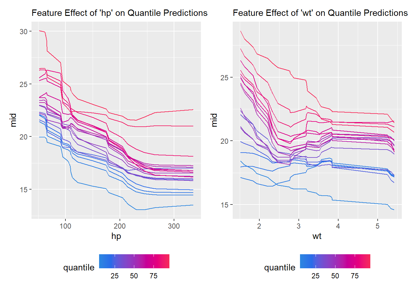
Instead of predicting the conditional mean, quantile regression predicts values at \(m\) different quantile levels (e.g., 50th, 75th, 95th, and 99th percentiles). Applying MID to this \(n \times m\) output matrix helps identify which variables drive the median behavior versus which variables govern extreme tail risks (e.g., the severity of unusually large claims).
Code
library(ranger)fit_rf <-ranger( mpg ~ .,data = mtcars,quantreg =TRUE)mid_rf <-interpret( mpg ~ .,data = mtcars,model = fit_rf,lambda =1,pred.args =list(type ="quantiles",quantiles =c(1:19/20),target =NULL# required for the current version of midr::get.yhat() ))labels(mid_rf) <-c(1:19/20) *100p1 <-ggmid(mid_rf, "hp", theme ="shap", intercept =TRUE) +labs(color ="quantile", subtitle ="Feature Effect of 'hp' on Quantile Predictions") +theme(legend.position ="bottom")p2 <-ggmid(mid_rf, "wt", theme ="shap", intercept =TRUE) +labs(color ="quantile", subtitle ="Feature Effect of 'wt' on Quantile Predictions") +theme(legend.position ="bottom")p1 + p2
Conclusion
In this notebook, we have demonstrated how Maximum Interpretation Decomposition (MID) bridges the gap between predictive performance and model transparency. By using the {midr} package, we successfully transformed a complex LightGBM model into a structured, additive representation.
Key takeaways include:
A pragmatic functional decomposition: MID is defined as the minimizer of the Uninterpreted Ratio (UR).
High-fidelity, inherently interpretable global surrogate: Fidelity is explicitly quantified by UR, providing a defensible basis for discussions with management, auditors, and regulators.
Highly extensible: It extends naturally to matrix-valued outputs, e.g., survival curves (SurvMID(t)).
Ready to use today: Available via {midr}, {midnight}, and {midlearn}.
As machine learning models become increasingly prevalent in insurance pricing and reserving, tools like MID will be essential for ensuring that our “black-boxes” remain accountable, reliable, and fundamentally understood.
{midlearn} (Scikit-learn Integration via Python): PyPI | GitHub
References
Asashiba, R., et al. (2025). midr: Learning from Black-Box Models by Maximum Interpretation Decomposition. arXiv:2506.08338.
Friedman, J. H. (2001). Greedy function approximation: A gradient boosting machine. The Annals of Statistics, 29(5), 1189–1232. doi:10.1214/aos/1013203451.
Apley, D. W., & Zhu, J. (2020). Visualizing the effects of predictor variables in black box supervised learning models. Journal of the Royal Statistical Society Series B, 82(4), 1059–1086. doi:10.1111/rssb.12377