`excess_plot()` creates a mean or median excess plot as a side-effect and returns the data frame invisibly.
Arguments
- x
a numeric vector.
- method
"mean" or "median".
- mode
"exact" or "interpolate".
- show_plot
logical.
- ...
optional arguments to be passed to the
plot()function, such asmain,xlab,ylab,col, etc.
Value
`excess_plot()` returns a data frame containing the data used for plotting.
If show_plot is TRUE, the data frame is returned invisibly.
Details
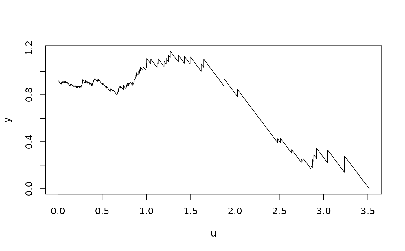
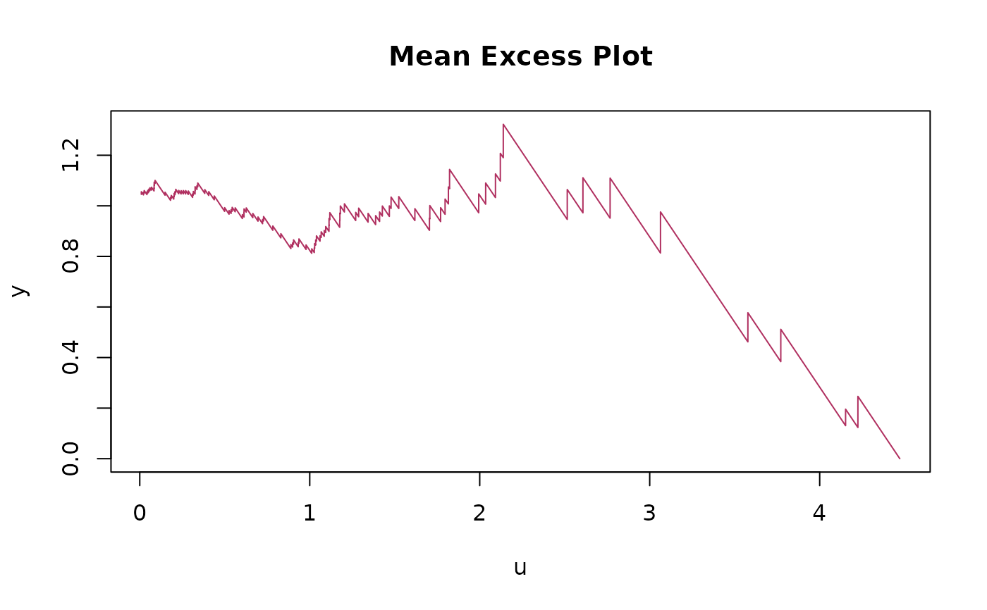
`excess_plot()` generates a mean or median excess plot, which is a key tool for visually assessing the tail behavior of a distribution.
Mean Excess Plot (MEP) represents the function \(e(u) = \mathrm{E}[\;\mathrm{X} - u\mid\mathrm{X} > u\;]\), i.e., the average of all exceedances over a given threshold u.
This plot helps in identifying the type of tail behavior.
An upward trend suggests a heavy-tailed distribution, a flat trend indicates an exponential distribution, and a downward trend points to a light-tailed distribution.
Median Excess Plot is similar to the MEP, but uses the median of the exceedances instead of the mean. This makes the plot more robust to outliers.