Going Beyond: Interpreting Survival Models

Introduction

Expanding Interpretability to Survival Analysis

We are thrilled to announce the release of {midr} 0.6.0. This update brings the core principles of the MID framework to a highly requested domain: Survival Analysis.

With this release, users can now decompose and interpret complex, “black-box” survival models—such as Random Survival Forests (RSF)—just as easily as standard regression and classification models.

Key new features in 0.6.0 include:

• Native Support for Survival Models: The interpret() function now natively supports some survival models including Cox proportional hazard models ({survival}) and random survival forests ({randomForestSRC}, {ranger}).

• Time-Dependent Sequence of MID Models: Because predicted survival probabilities change over time, {midr} now calculates and returns an array of time-varying MID surrogate models.

Example

# required packages
library(survival)
library(randomForestSRC)
library(midr)

library(ggplot2)
library(gridExtra)
library(patchwork)

data(flchain, package = "survival")

Here is a look at how {midr} 0.6.0 interprets a Random Survival Forest model using the flchain dataset.

Predictive Modeling

# predictive modeling: random survival forest
rsf_model <- rfsrc(
  Surv(futime, death) ~ age + sex + sample.yr + kappa + lambda, 
  data = flchain, 
  ntree = 100,
  nodesize = 20,
  na.action = "na.impute"
)

rsf_model

                         Sample size: 7874
                    Number of deaths: 2169
                     Number of trees: 100
           Forest terminal node size: 20
       Average no. of terminal nodes: 245.64
No. of variables tried at each split: 3
              Total no. of variables: 5
       Resampling used to grow trees: swor
    Resample size used to grow trees: 4976
                            Analysis: RSF
                              Family: surv
                      Splitting rule: logrank *random*
       Number of random split points: 10
                          (OOB) CRPS: 463.86434184
             (OOB) standardized CRPS: 0.09280999
   (OOB) Requested performance error: 0.29755615

Surrogate Modeling

# surrogate modeling
mid_model <- interpret(
  Surv(futime, death) ~ (age + sex + sample.yr + kappa + lambda) ^ 2, 
  data = flchain,
  model = rsf_model,
  lambda = .05,
  na.action = na.pass
)

mid_model

Call:
interpret(formula = Surv(futime, death) ~ (age + sex + sample.yr +
 kappa + lambda)^2, data = flchain, model = rsf_model, na.action = na.pass,
 lambda = 0.05)

Model Class: rfsrc, grow, surv

Intercept: 0.99963, 0.99558, 0.99345, ...

Main Effects:
5 main effect terms

Interactions:
10 interaction terms

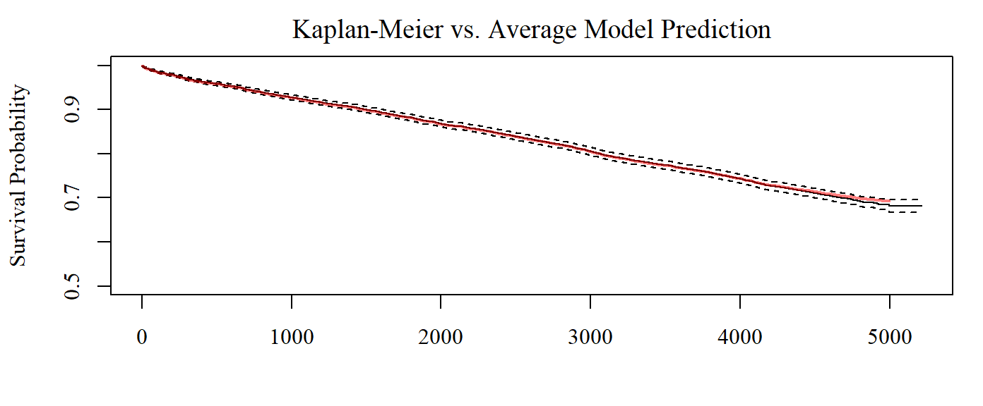
Uninterpreted Variation Ratio: 0.78773, 0.61879, 0.44844, ...

Intercept

Baseline survival probabilities, i.e. the average predicted survival probabilities, are stored as $intercept.

Here, we compare the intercepts with the Kaplan-Meier curve.

km_fit <- survfit(
  Surv(futime, death) ~ 1, data = flchain
)

par.midr()

plot(
  km_fit, 
  main = "Kaplan-Meier vs. Average Model Prediction",
#  xlab = "Days from Sample Collection", 
  ylab = "Survival Probability",
  ylim = c(0.5, 1.0)
)

lines(
  x = as.numeric(labels(mid_model)),
  y = mid_model$intercept,
  col = "#FF000080",
  lwd = 2
)

Uninterpreted Variation Ratio

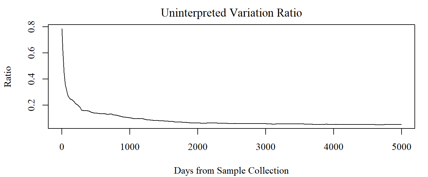
Since {midr} fits as many models as the number of time periods of interest, the uninterpreted variation ratio changes with time.

par.midr()

plot(
  x = as.numeric(labels(mid_model)),
  y = mid_model$ratio,
  type = "l",
  main = "Uninterpreted Variation Ratio",
  ylab = "Ratio",
  xlab = "Days from Sample Collection"
)

Feature Importance

Just as survival probabilities change over time, so does the relative impact of each predictor. What strongly influences short-term survival may not be the primary driver of long-term outcomes.

For the MID-based surrogate models, mid.importance() function captures this dynamic behavior, allowing you to visualize how the importance of individual features and their interactions evolves across the specified time horizon.

imp <- mid.importance(mid_model)

p <- ggmid(
  imp,
  theme = "magma",
  terms = rev(head(mid.terms(imp), 10))
) +
  theme(legend.position = "none") +
  labs(subtitle = "Feature Importance") +
  coord_flip()

q <- ggmid(
  imp,
  type = "series",
  theme = "Tableau 10",
  terms = mid.terms(imp, interactions = FALSE),
  linewidth = 3/4
) +
  labs(x = "Days from Sample Collection") +
  theme(legend.position = "bottom")

p / q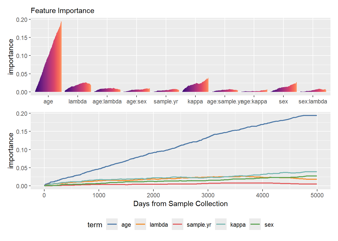

p1 <- ggmid(imp[50], fill = "steelblue") +
  labs(subtitle = paste("Feature Importance on Day", labels(mid_model)[50]))
p2 <- ggmid(imp[100], fill = "maroon") +
  labs(subtitle = paste("Feature Importance on Day", labels(mid_model)[100]))
p1 + p2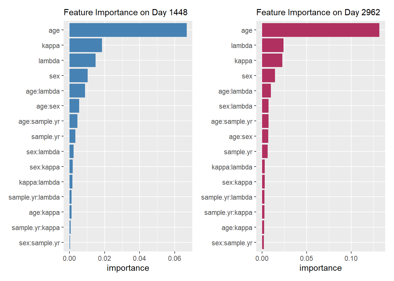

Feature Effects

Beyond knowing which features matter, it is crucial to understand how they influence predictions over time. By evaluating the component functions, you can extract the estimated main and interaction effects on survival probabilities. This provides a clear, time-varying view of partial dependencies, showing exactly how different values of a feature shift the survival curve.

plots <- mid.plots(
  mid_model,
  terms = c("age", "lambda", "kappa", "sex"),
  type = "series",
  theme = "mako",
  resolution = 100,
  intercept = TRUE,
  limits = c(-0.05, 1.05)
)

plots[[1]] <- plots[[1]] +
  labs(subtitle = "Feature Effect on Survival Probability")
plots[[4]] <- plots[[4]] +
  labs(x = "Days from Sample Collection")
plots[[1]] / plots[[2]] / plots[[3]] / plots[[4]]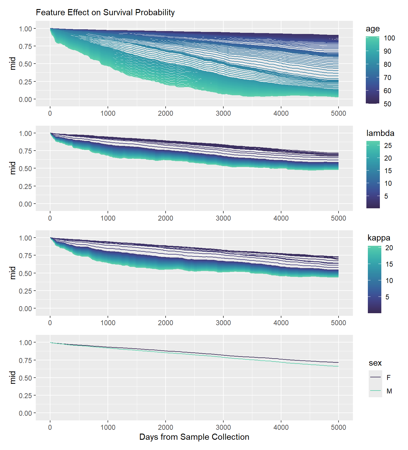

Breakdown of Effects

To build trust in clinical or business applications, we often need to explain individual predictions.

The mid.breakdown() function zooms in on a single observation, decomposing that specific patient’s predicted survival curve into additive contributions from the baseline and each feature. This makes it intuitively clear exactly which risk factors are driving an individual’s prognosis at any given moment.

brk <- mid.breakdown(mid_model, data = flchain[1 ,])

p <- ggmid(
  brk,
  theme = "cividis",
  terms = rev(head(mid.terms(imp, interactions = FALSE)))
) +
  theme(legend.position = "none") +
  labs(subtitle = "Breakdown of Prediction") +
  coord_flip()

q <- ggmid(
  brk,
  type = "series",
  theme = "Tableau 10",
  terms = mid.terms(imp, interactions = FALSE),
  linewidth = 3/4
) +
  labs(x = "Days from Sample Collection") +
  theme(legend.position = "bottom")

p / q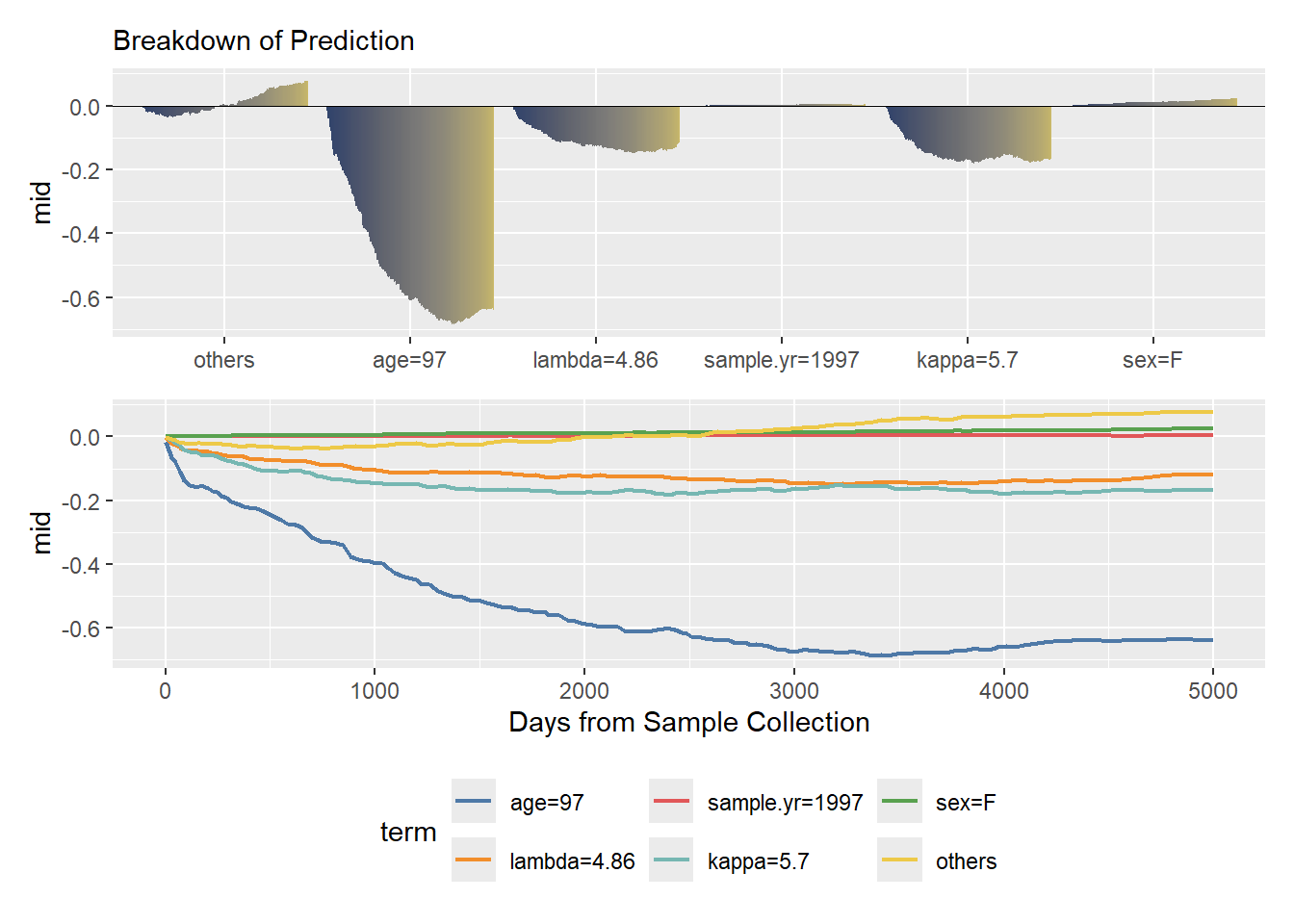

p1 <- ggmid(brk[50], fill = "steelblue") +
  labs(subtitle = paste("Breakdown on Day", labels(mid_model)[50]))
p2 <- ggmid(brk[100], fill = "maroon") +
  labs(subtitle = paste("Breakdown on Day", labels(mid_model)[100]))
p1 + p2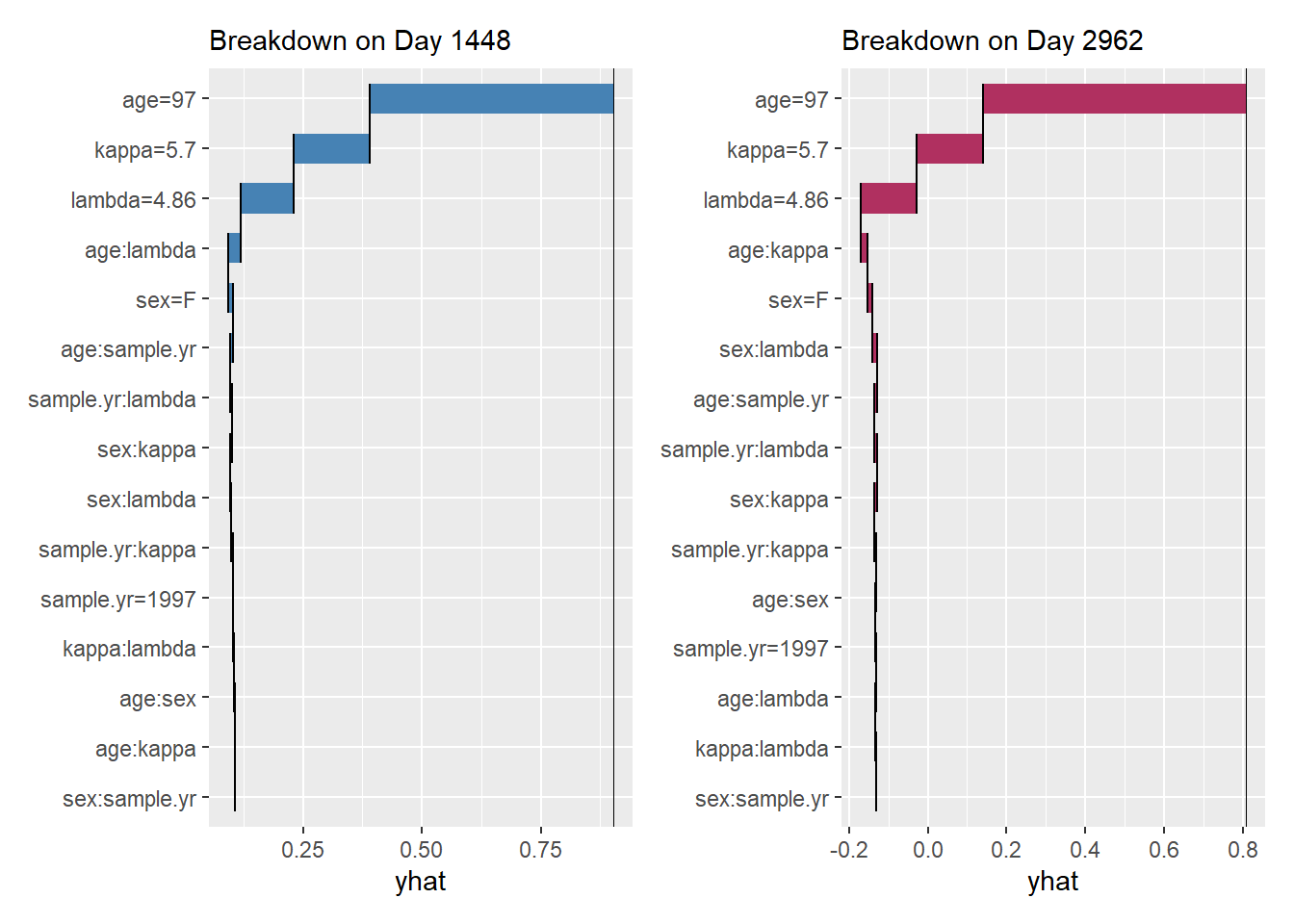

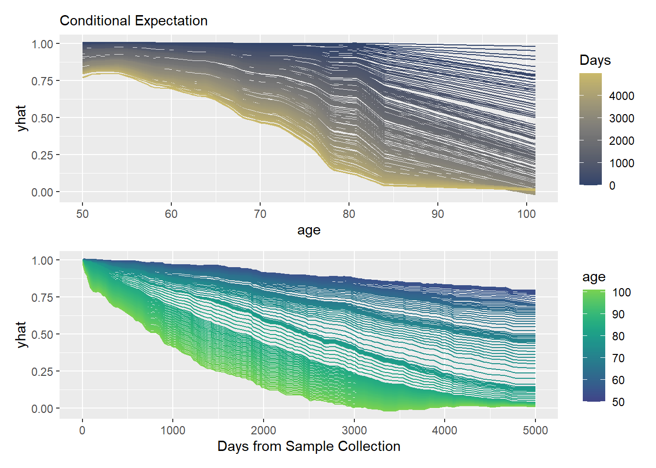
Conditional Expectation

For a more granular look at how a model behaves, Individual Conditional Expectation (ICE) plots are an invaluable tool.

Using mid.conditional(), you can explore counterfactual “what-if” scenarios—visualizing how modifying a specific feature alters the predicted survival outcome for an individual patient. This highlights the change of feature effects in time.

con <- mid.conditional(mid_model, variable = "age", data = flchain[100, ])
p1 <- ggmid(con, theme = "cividis") +
  labs(subtitle = "Conditional Expectation", color = "Days")
p2 <- ggmid(con, theme = "viridis", type = "series") +
  labs(x = "Days from Sample Collection")
p1 / p2