In modern actuarial science, there is an inherent tension between predictive accuracy and model transparency. While ensemble tree-based models like Gradient Boosting Machines (GBMs) frequently outperform traditional Generalized Linear Models (GLMs), their “black-box” nature presents significant hurdles for model governance, regulatory compliance, and price filing.
This notebook demonstrates a solution using Maximum Interpretation Decomposition (MID) via the {midr} and {midnight} packages in R.
WarningCompatibility Notice
This article relies on features introduced in midr (>= 0.6.0) and midnight (>= 0.1.1.902). Please ensure your packages are up to date. Some visualization arguments are not available in earlier versions.
What is MID?
MID is a functional decomposition method that deconstructs a black-box prediction function \(f(\mathbf{X})\) into several interpretable components: an intercept \(g_\emptyset\), main effects \(g_j(X_j)\), and second-order interactions \(g_{jk}(X_j, X_k)\), minimizing the squared residuals \(\mathbf{E}\left[g_D(\mathbf{X})^2\right]\):
To ensure the uniqueness and identifiability of each component, MID imposes centering and probability-weighted minimum-norm constraints on the decomposition.
By approximating a black-box model with this surrogate structure, we can derive a representation that retains the superior predictive power of machine learning models without sacrificing actuarial transparency. Furthermore, it allows us to quantify the “uninterpreted” variance, i.e., the portion of the model’s logic that can’t be captured by low-order effects, via the residual term \(g_D(\mathbf{X})\).
Setting Up
We begin by setting up the environment and loading the necessary libraries.
Code
# data manipulationlibrary(arrow)library(dplyr)# predictive modelinglibrary(gam)library(lightgbm)# surrogate modelinglibrary(midr)library(midnight)nightfall(methods =TRUE, solvers =FALSE, themes =FALSE)# visualizationlibrary(ggplot2)library(gridExtra)# load training and testing datasetstrain <-read_parquet("../data/train.parquet")test <-read_parquet("../data/test.parquet")
A key component of our evaluation is the Weighted Mean Poisson Deviance defined as follows:
We first fit a GAM to establish a transparent benchmark. Since GAMs are additive by design, they provide a “ground truth” model structure to be recovered by the functional decomposition.
This metric represents the proportion of the black-box model’s variance that is not captured by the additive components of the MID model. The R-squared score, \(\mathbf{R}^2(f,g) = 1 - \mathbf{U}(f,g)\), is a standard measure for this purpose. However, it is important to note that this \(\mathbf{R}^2\) measures the fidelity to the black-box model \(f\), rather than the predictive accuracy relative to the ground truth observations as is typically the case with standard R-squared.
In the {midr} package, the summary output includes this ratio calculated on the training set. For models with non-linear links (e.g., Poisson regression), the “working” ratio is computed on the scale of the link function (e.g., \(\log\) scale).
To rigorously confirm the model fidelity, it is recommended to evaluate these metrics on a separate testing set. This ensures that the surrogate model is not just over-fitting the training predictions but has truly captured the underlying functional structure.
As shown by the high \(\mathbf{R}^2\) score, the MID surrogate achieves near-perfect fidelity. This level of agreement justifies using the MID components (main effects and interactions) as a reliable lens through which to interpret the original black-box model’s behavior.
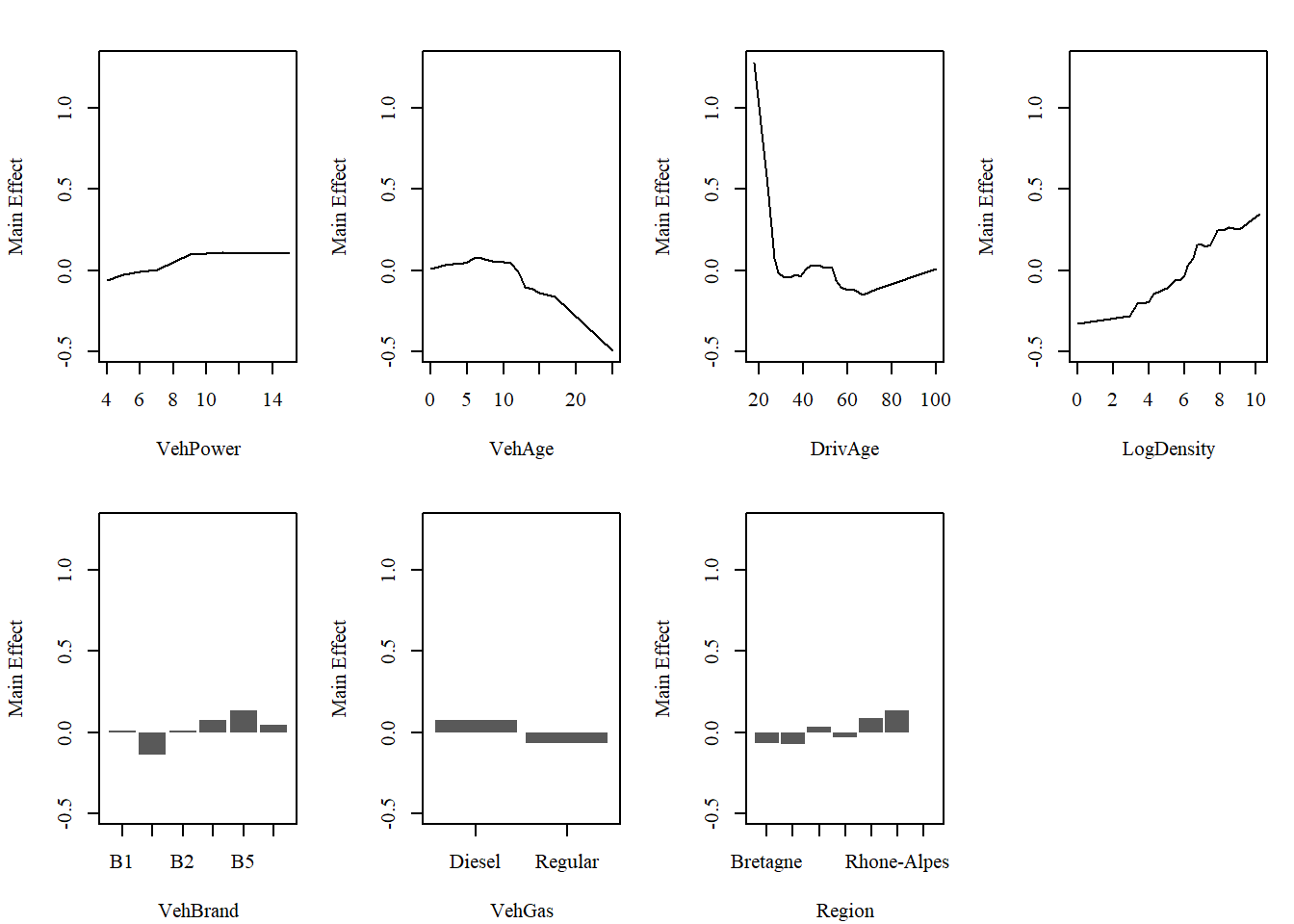
Feature Effects
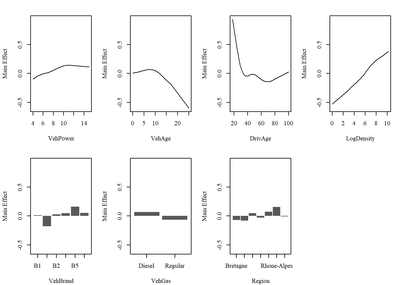
Visualizing the functional behavior of each component allows for a direct comparison between the MID surrogate’s decomposition and the original GAM’s structure.
MID Surrogate
Code
# main effects of MID surrogatepar.midr(mfrow =c(2, 4))mid.plots(mid_gam, engine ="graphics", ylab ="Main Effect")
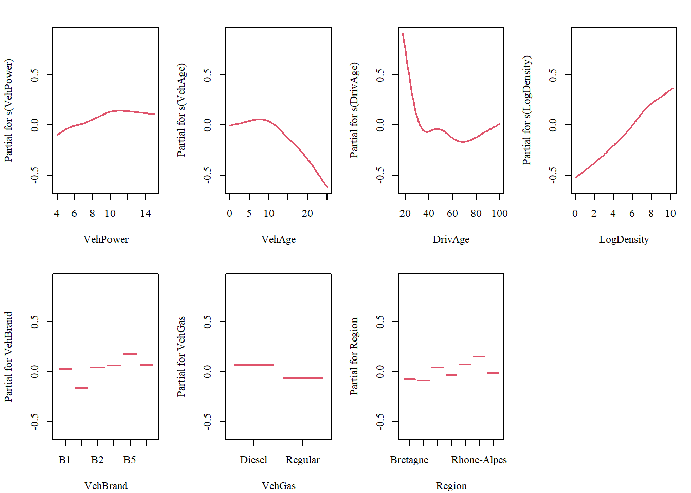
Original GAM
Code
# feature effects of GAMpar.midr(mfrow =c(2, 4))termplot(fit_gam)
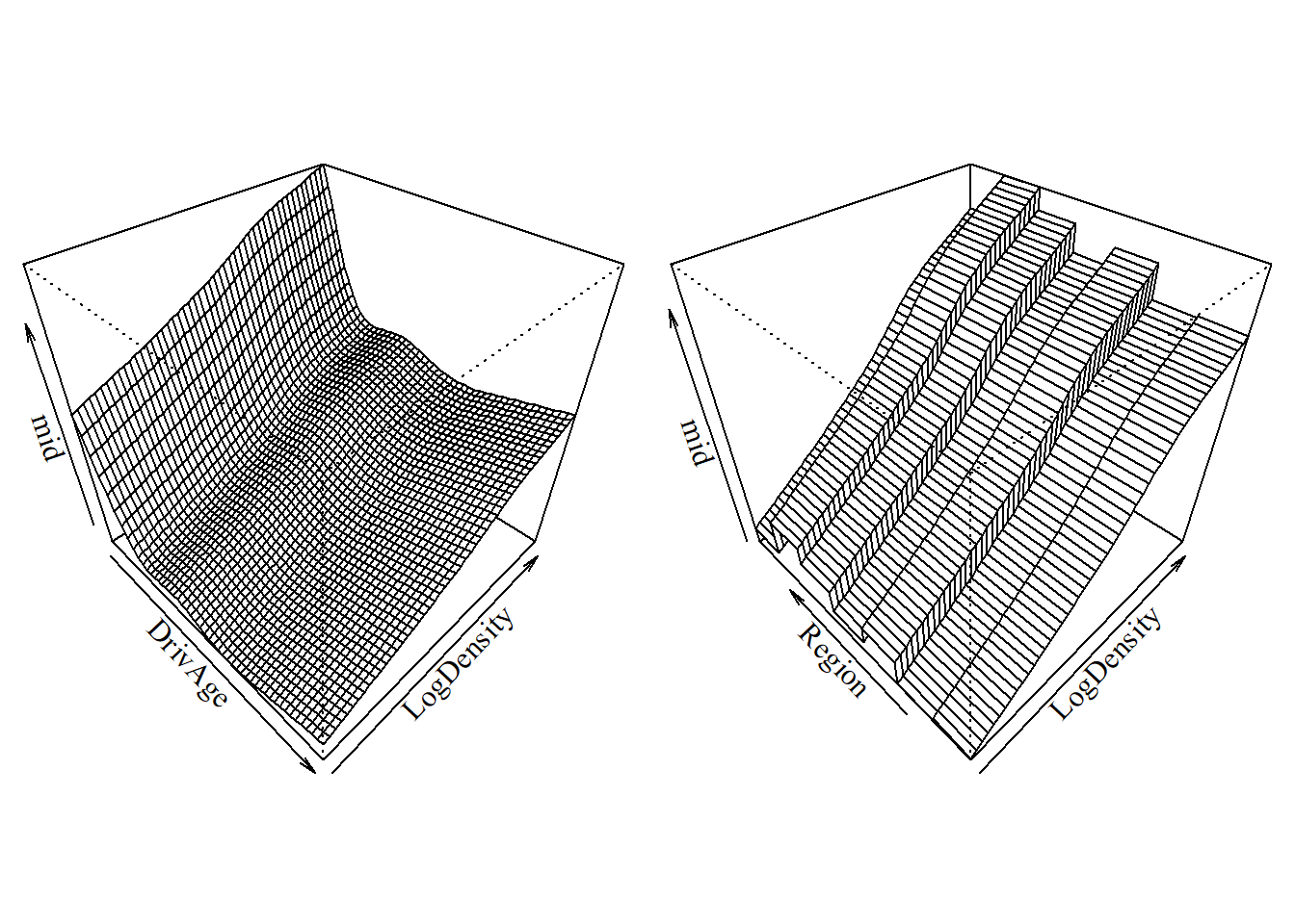
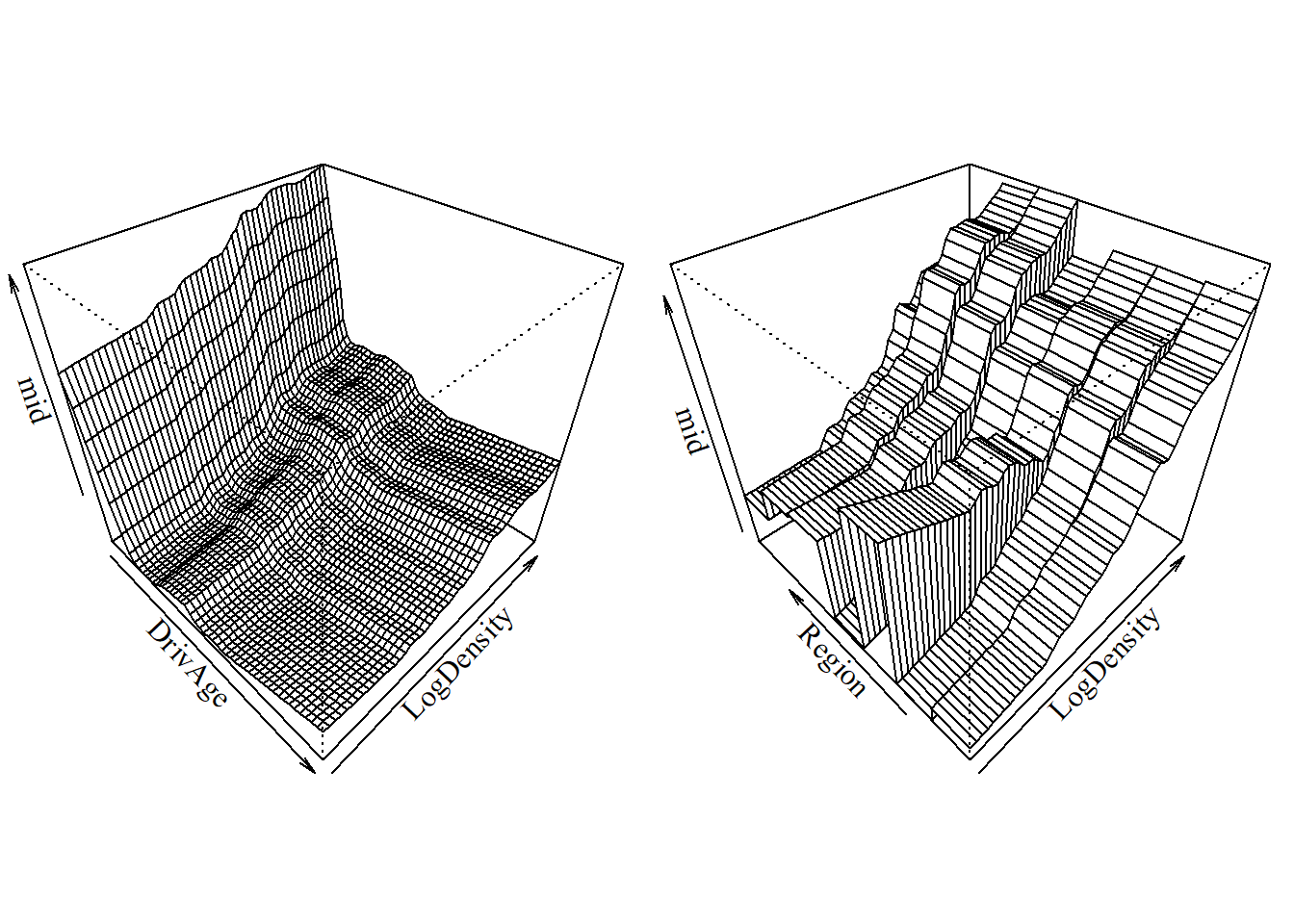
Furthermore, we can visualize the joint effects of feature pairs as 3D prediction surfaces using the S3 method for the persp() function.
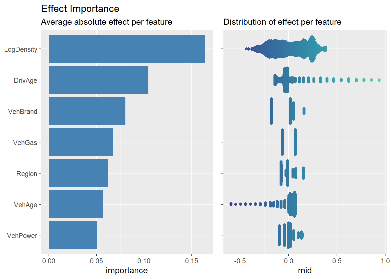
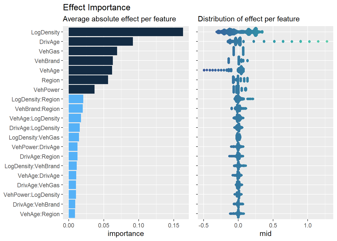
Beyond simple plots for feature effects, {midr} provides a suite of diagnostic tools. First, the Effect Importance of a term \(j\) is defined as the mean absolute contribution of that term across the population:
imp_gam <-mid.importance(mid_gam, data = train, max.nsamples =2000)grid.arrange(nrow =1, widths =c(5, 4),ggmid(imp_gam, fill ="steelblue") +labs(title ="Effect Importance",subtitle ="Average absolute effect per feature"),ggmid(imp_gam, type ="beeswarm", theme ="mako@div") +labs(title ="",subtitle ="Distribution of effect per feature") +scale_y_discrete(labels =NULL) +theme(legend.position ="none"))
For interaction terms, the importance is similarly calculated using \(g_{jk}(X_j, X_k)\). This metric allows us to rank features by their average influence on the model’s predictions.
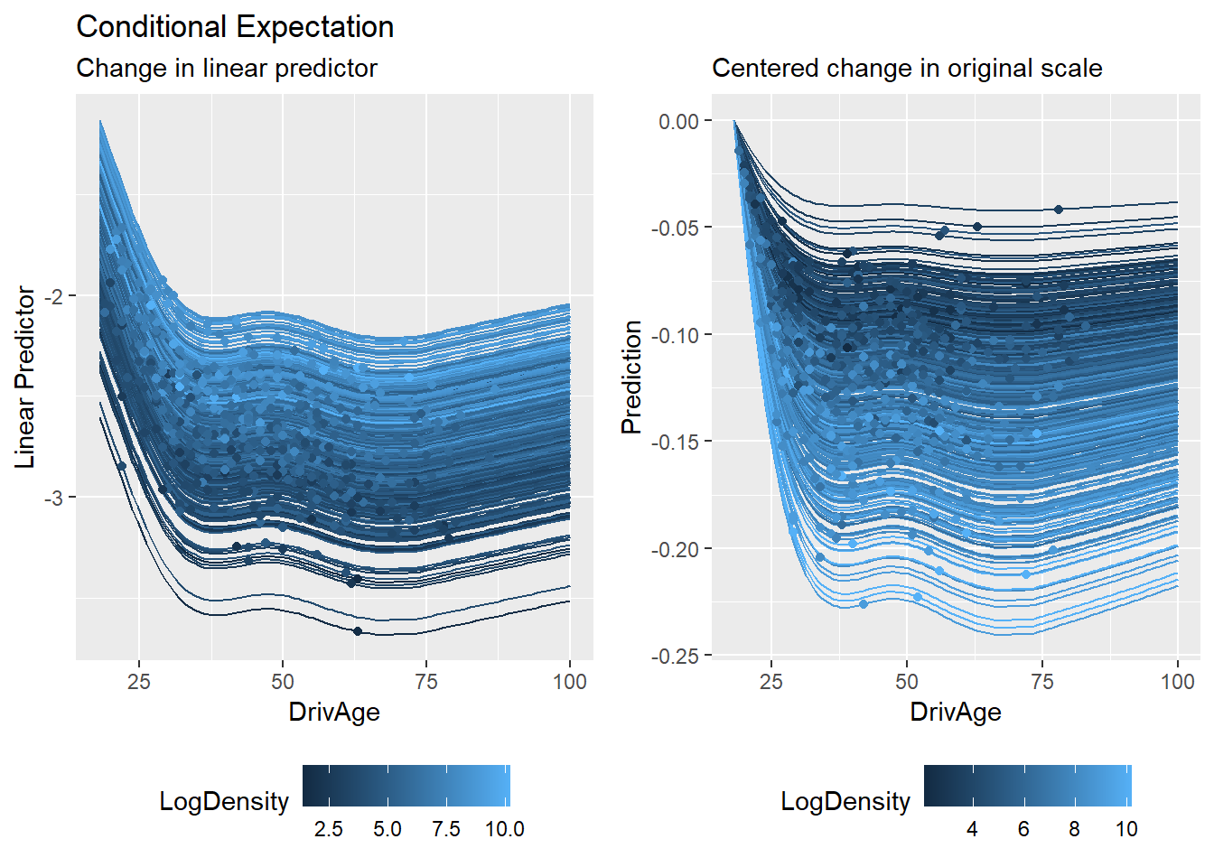
Conditional Expectation
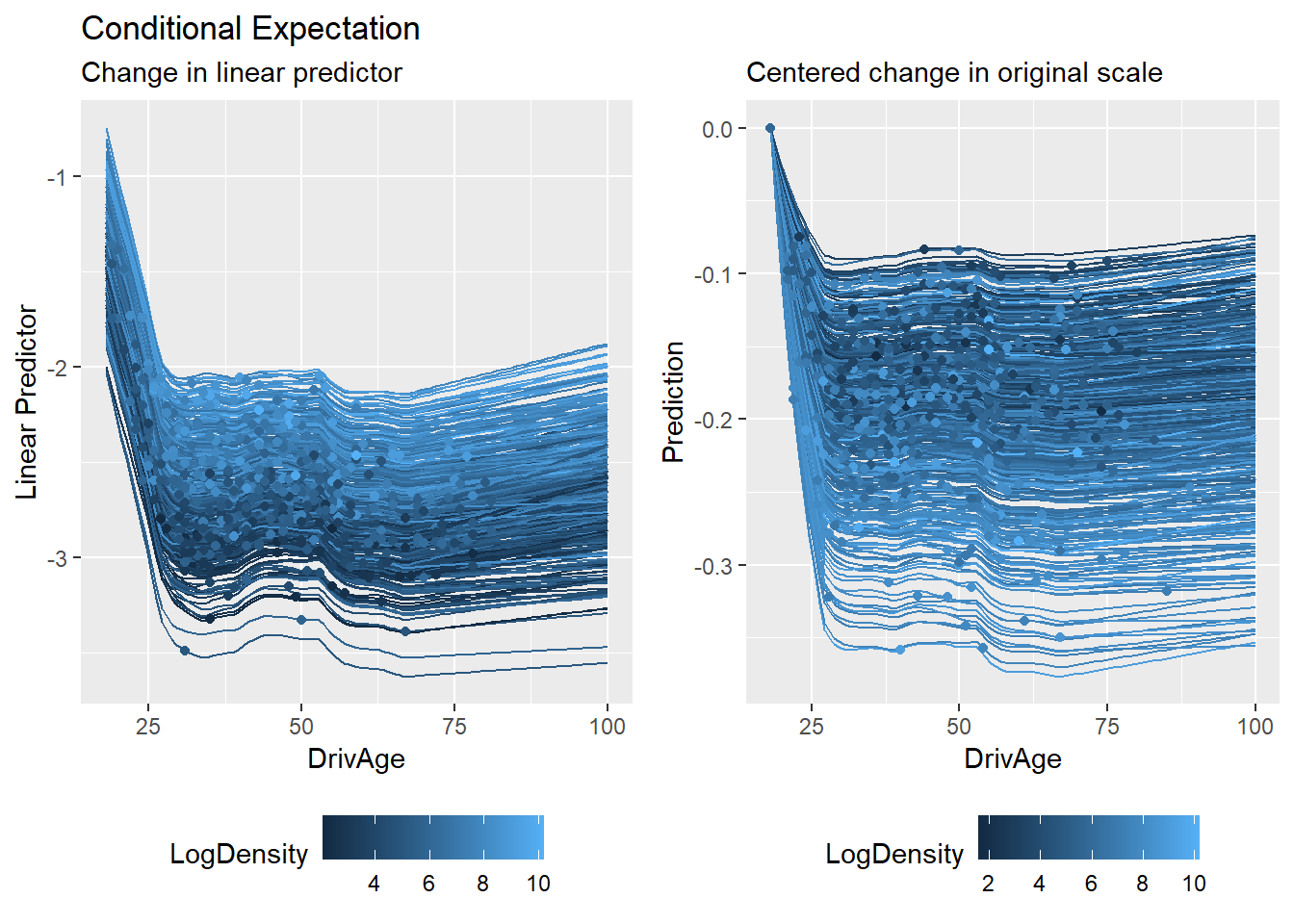
Second, we can explore Individual Conditional Expectations (ICE). In the MID framework, the ICE for a feature \(j\) and a specific observation \(i\) is the expected value of the prediction as \(X_j\) varies, while keeping other features fixed at their observed values \(\mathbf{x}_{i,\setminus j}\):
ice_gam_link <-mid.conditional(mid_gam, type ="link", variable ="DrivAge")ice_gam <-mid.conditional(mid_gam, variable ="DrivAge")grid.arrange(nrow =1,ggmid(ice_gam_link, var.color = LogDensity) +theme(legend.position ="bottom") +labs(y ="Linear Predictor",title ="Conditional Expectation",subtitle ="Change in linear predictor"),ggmid(ice_gam, type ="centered", var.color = LogDensity) +theme(legend.position ="bottom") +labs(y ="Prediction", title ="",subtitle ="Centered change in original scale"))
Unlike standard black-box models, MID’s low-order structure allows us to compute these expectations efficiently and interpret the variation across curves (the “thickness” of the ICE plot) as a direct consequence of specified interaction terms \(g_{jk}\).
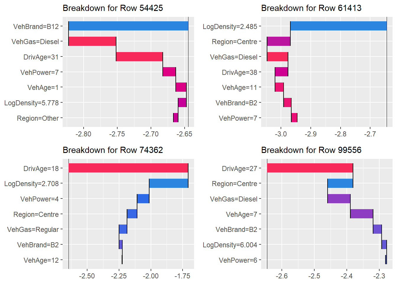
Additive Attribution
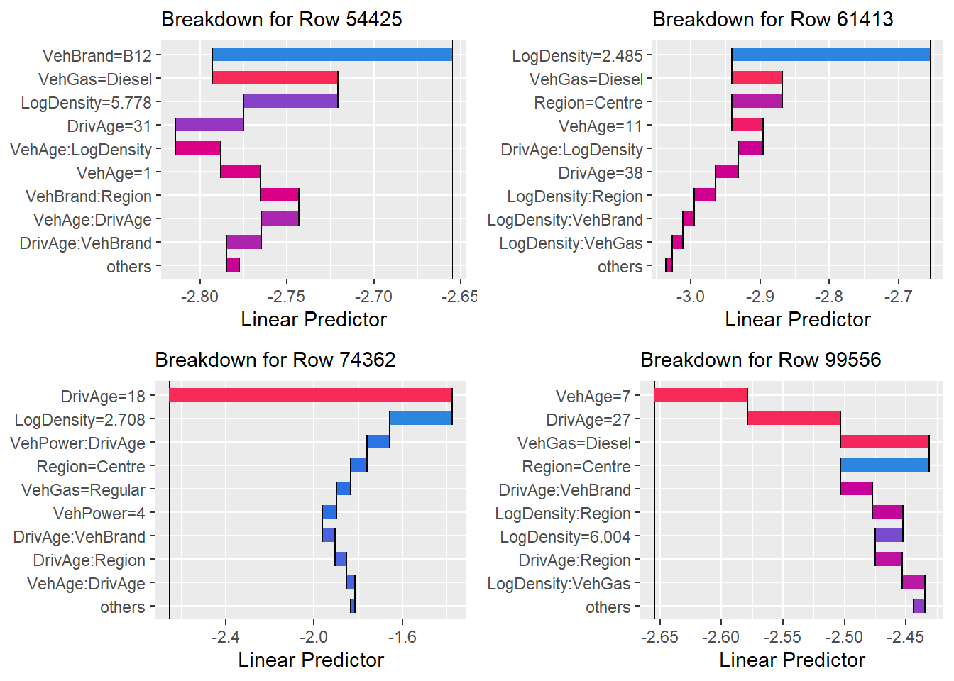
Third, we perform instance-level explanation through an Additive Breakdown of the prediction. For any single observation \(\mathbf{x}\), the MID surrogate’s prediction \(g(\mathbf{x})\) is decomposed into the exact sum of its functional components:
By visualizing these contributions in a waterfall plot, we can identify which specific risk factors or interaction effects drove the prediction for a particular instance, such as a high-risk policyholder.
The Black-Box: LightGBM
While GAMs are transparent, GBMs such as LightGBM often yield superior predictive power by capturing high-order interactions. However, this accuracy comes at the cost of being a black box.
We use {midr} to replicate the LightGBM model. By including interaction terms in the model formula, we allow the surrogate to capture the joint relationships that the GBM has learned. The goal is to approximate the LightGBM function \(f_{LGB}(\mathbf{x})\) with our interpretable structure \(g(\mathbf{x})\):
Including all second-order interactions using the (...)^2 syntax results in \(p(p-1)/2\) interaction terms. For high-dimensional data, this can be memory-intensive. Users should ensure sufficient RAM is available or consider limiting the formula to the most relevant features, or using a subset of the training set.
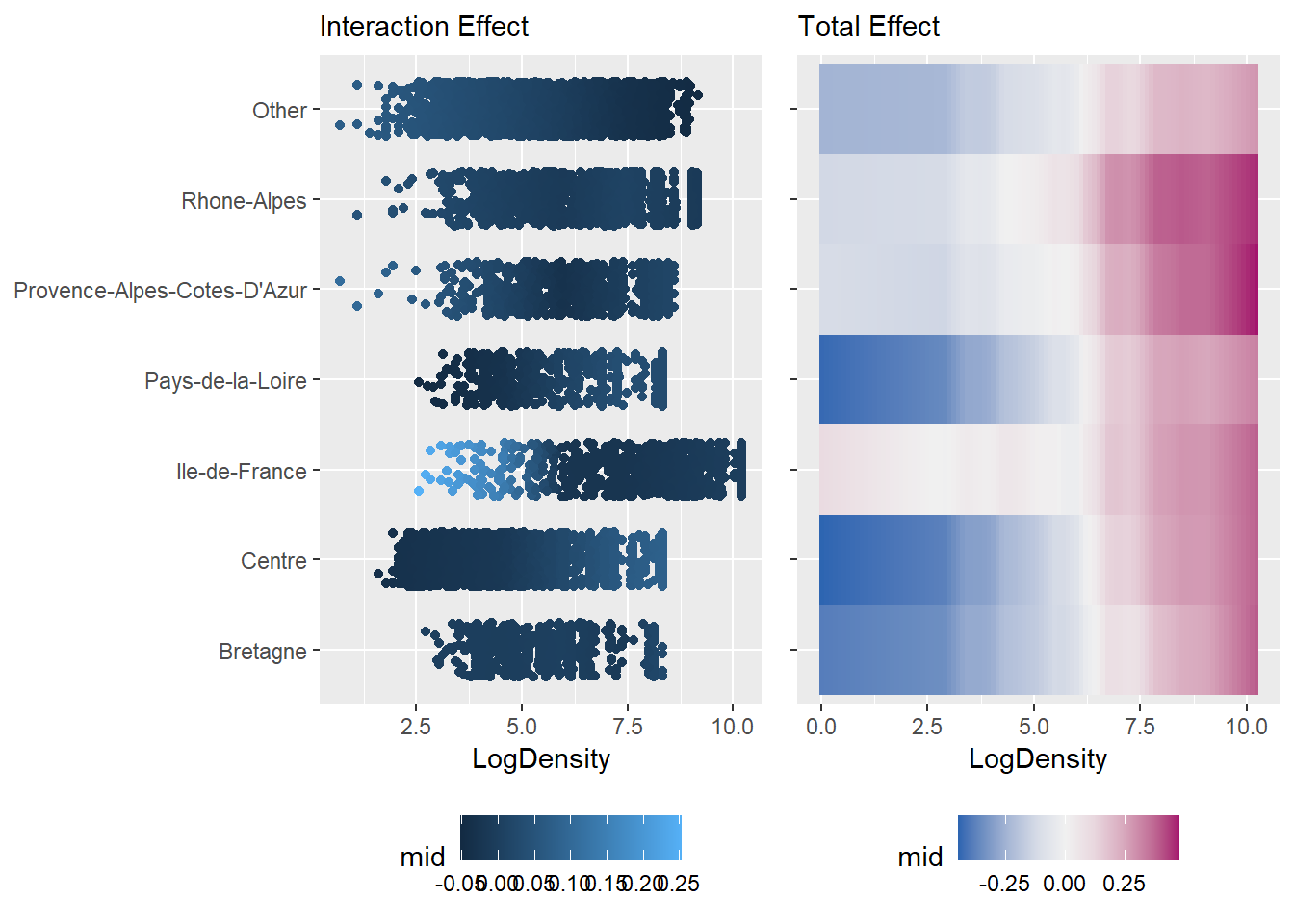
A key advantage of {midr} is its ability to isolate interaction effects \(g_{jk}\) from main effects \(g_j\). This is particularly useful to understand the joint impact of two variables (e.g., Region and LogDensity).
To rank the influence of each component discovered in the LightGBM model, we calculate the Effect Importance, defined as the average absolute contribution.
Code
imp_lgb <-mid.importance(mid_lgb, data = train, max.nsamples =2000)grid.arrange(nrow =1, widths =c(4, 3),ggmid(imp_lgb, theme ="bluescale@qual", max.nterms =20) +labs(title ="Effect Importance",subtitle ="Average absolute effect per feature") +theme(legend.position ="none"),ggmid(imp_lgb, type ="beeswarm", theme ="mako@div", max.nterms =20) +labs(title ="",subtitle ="Distribution of effect per feature") +scale_y_discrete(labels =NULL) +theme(legend.position ="none"))
Conditional Expectation
We further explore the model’s behavior using the ICE plot. In the MID framework, the variation in ICE curves for a feature \(j\) is explicitly governed by the interaction terms \(g_{jk}\) identified from the LightGBM model.
Code
ice_lgb_link <-mid.conditional(mid_lgb, type ="link", variable ="DrivAge")ice_lgb <-mid.conditional(mid_lgb, variable ="DrivAge")grid.arrange(nrow =1,ggmid(ice_lgb_link, var.color = LogDensity) +theme(legend.position ="bottom") +labs(y ="Linear Predictor",title ="Conditional Expectation",subtitle ="Change in linear predictor"),ggmid(ice_lgb, type ="centered", var.color = LogDensity) +theme(legend.position ="bottom") +labs(y ="Prediction", title ="",subtitle ="Centered change in original scale"))
Additive Attribution
Finally, we perform an Additive Breakdown for individual predictions. This provides an exact allocation of the LightGBM’s prediction into the terms of our surrogate model.
In this notebook, we have demonstrated how Maximum Interpretation Decomposition (MID) bridges the gap between predictive performance and model transparency. By using the {midr} package, we successfully transformed a complex LightGBM model into a structured, additive representation.
While the surrogate model fidelity may not always be perfect, the crucial advantage lies in our ability to quantify its limitations. Through the uninterpreted variation ratio, we can directly assess the complexity of the black-box model. If the fidelity is lower than expected, it serves as a diagnostic signal that the original model relies on high-order interactions or structural complexities that extend beyond second-order effects.
Knowing the extent of this “unexplained” variance is far more valuable than operating in the dark. It allows actuaries to make informed decisions about whether the additional complexity of a black-box model is justified by its performance, or if a more transparent structure is preferable for regulatory and risk management purposes.
As machine learning models become increasingly prevalent in insurance pricing and reserving, tools like MID will be essential for ensuring that our “black-boxes” remain accountable, reliable, and fundamentally understood.