Introduction to midnight: Core Modeling and Fast Solvers

The midnight package is designed to provide robust modeling capabilities and highly optimized solvers, working seamlessly alongside the midr package. The core philosophy of midnight revolves around its two main functionalities:

1. mid_reg(): A seamless tidymodels (parsnip) interface for intuitive model specification.

2. fastLmMatrix(): High-performance multivariate least squares solvers designed for speed and efficiency.

In addition to these core computational features, the package offers advanced visualization tools and integrated color themes.

The Tidymodels Interface

midnight fully integrates with the tidymodels ecosystem. The mid_reg() function allows you to specify models using the familiar parsnip syntax, enabling pipeline-based workflows for model fitting and hyperparameter tuning.

library(midr)
library(midnight)
library(parsnip)
library(ggplot2)
library(patchwork)

# fitting a model with interaction using mid_reg()
mid <- mid_reg(
  params_main = 50, # k
  penalty = 5 # lambda
) |>
  fit(Ozone ~ (Wind + Solar.R) ^ 2, na.omit(airquality))

mid
#> parsnip model object
#> 
#> 
#> Call:
#> interpret(formula = Ozone ~ (Wind + Solar.R)^2, data = data,
#>  model = NULL, weights = NULL, k = 50, k2 = NULL, lambda = 5,
#>  terms = terms)
#> 
#> Intercept: 42.099
#> 
#> Main Effects:
#> 2 main effect terms
#> 
#> Interactions:
#> 1 interaction term
#> 
#> Uninterpreted Variation Ratio: 0.33087

High-Performance Least Square Solvers

For situations requiring fitting a surrogate model for multivariate responses, midnight provides highly optimized OLS solvers. You can compare standard RcppEigen implementations with the matrix-based solvers provided by midnight.

# standard RcppEigen solver
fit1 <- RcppEigen::fastLm(
  Ozone ~ Wind + Solar.R, na.omit(airquality)
)
print(as.matrix(fit1$coefficients))
#>                   [,1]
#> (Intercept) 77.2460424
#> Wind        -5.4017973
#> Solar.R      0.1003506
fit2 <- RcppEigen::fastLm(
  Temp ~ Wind + Solar.R, na.omit(airquality)
)
# fastLmMatrix
print(as.matrix(fit2$coefficients))
#>                    [,1]
#> (Intercept) 85.70227521
#> Wind        -1.25187025
#> Solar.R      0.02453254
fit3 <- fastLmMatrix(
  cbind(Ozone, Temp) ~ Wind + Solar.R, na.omit(airquality)
)
print(fit3$coefficients)
#>                  Ozone        Temp
#> (Intercept) 77.2460424 85.70227521
#> Wind        -5.4017973 -1.25187025
#> Solar.R      0.1003506  0.02453254

Furthermore, you can globally override the default Least Squares Solvers used in mid_reg() (and interpret()) to leverage this speed boost across your entire modeling pipeline by using nightfall().

# activate midnight package
nightfall()

mids <- mid_reg(
  params_main = 50, # k
  penalty = 5 # lambda
) |>
  fit(cbind(Ozone, Temp) ~ (Wind + Solar.R) ^ 2, airquality)
#> custom solver 'qr' is used

mids
#> parsnip model object
#> 
#> 
#> Call:
#> interpret(formula = cbind(Ozone, Temp) ~ (Wind + Solar.R)^2,
#>  data = data, model = NULL, weights = NULL, k = 50, k2 = NULL,
#>  lambda = 5, terms = terms)
#> 
#> Intercept: 42.099, 77.793
#> 
#> Main Effects:
#> 2 main effect terms
#> 
#> Interactions:
#> 1 interaction term
#> 
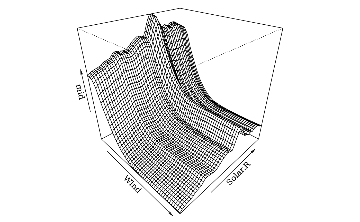
#> Uninterpreted Variation Ratio: 0.33087, 0.52745

New Visualization Styles

To understand the output of mid_reg(), midnight provides S3 methods for MID models like persp.mid() and ggmid.midimp(), which is activated when nightfall() is called. These methods help translate complex model outputs into interpretable insights.

Variable Importance

Using ggmid(type = 'beeswarm'), as well as 'violinplot' or 'sinaplot', you can effortlessly plot feature importance distributions to understand the impact of individual variables and their interactions.

imp <- mid.importance(mid$fit, data = airquality)
p1 <- ggmid(imp, type = "beeswarm", theme = "Hokusai3") +
  theme(legend.position = "bottom")
p2 <- ggmid(imp, type = "violin", theme = "moon") +
  theme(legend.position = "bottom")
p1 + p2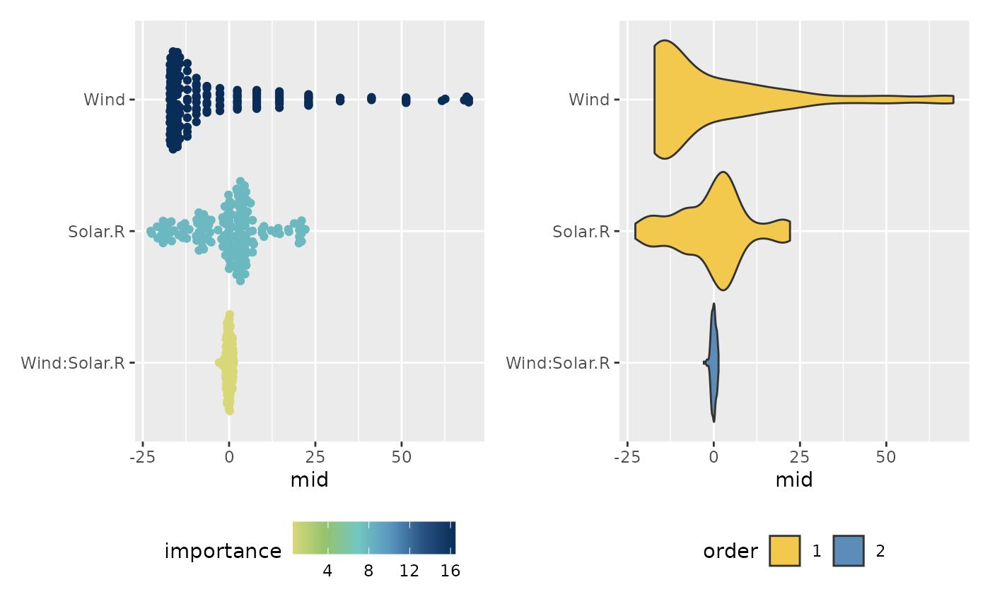

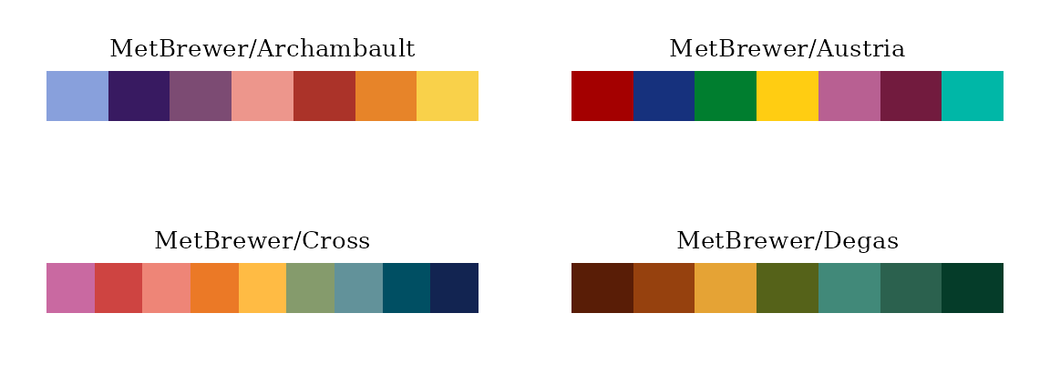
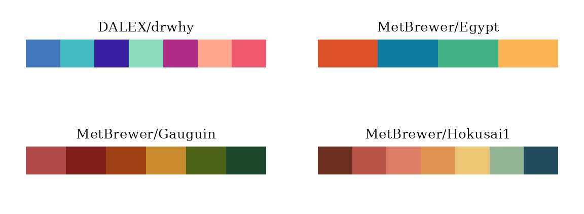
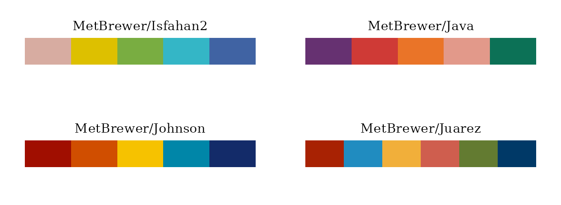
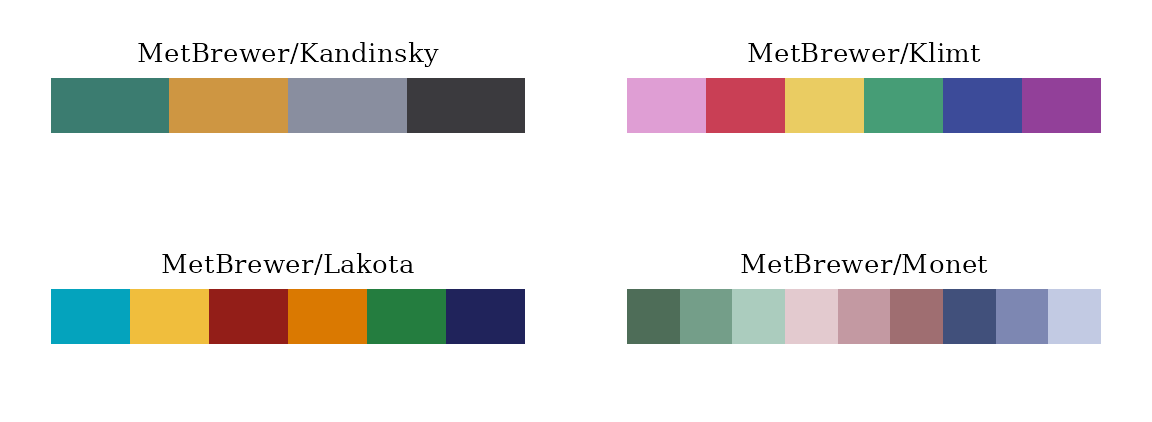
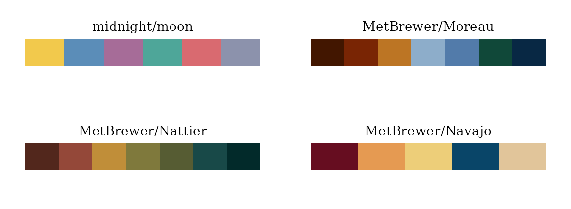
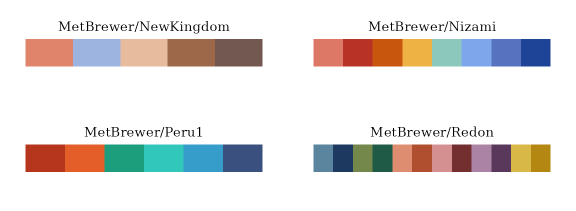
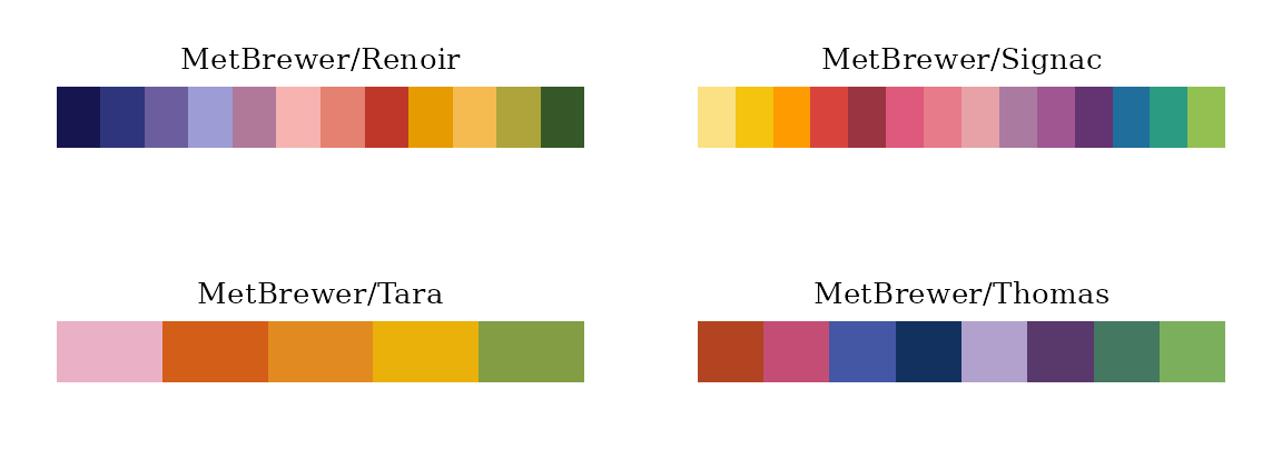
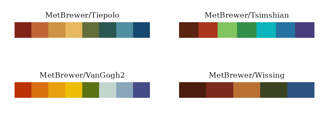
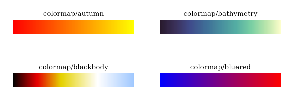
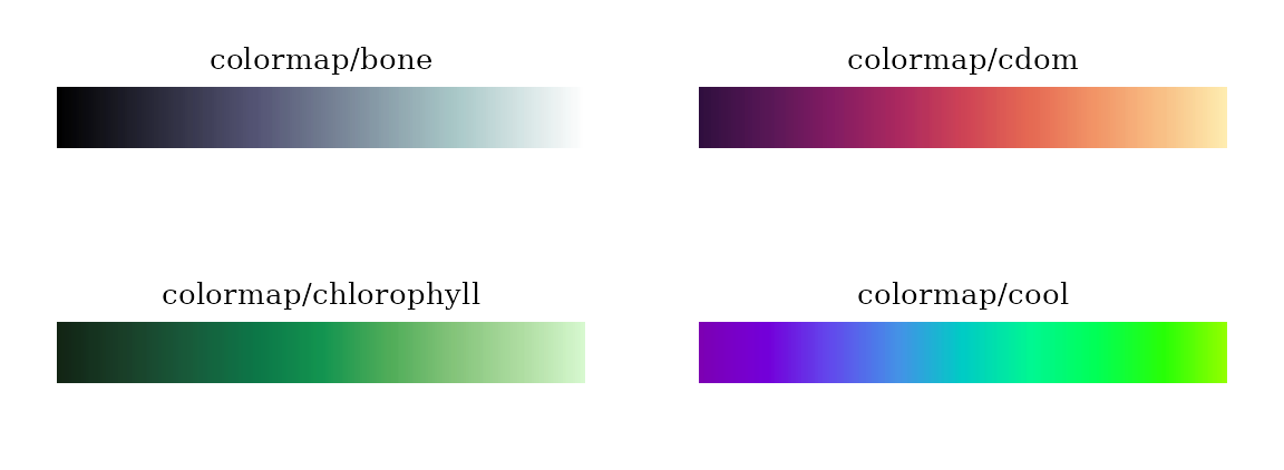
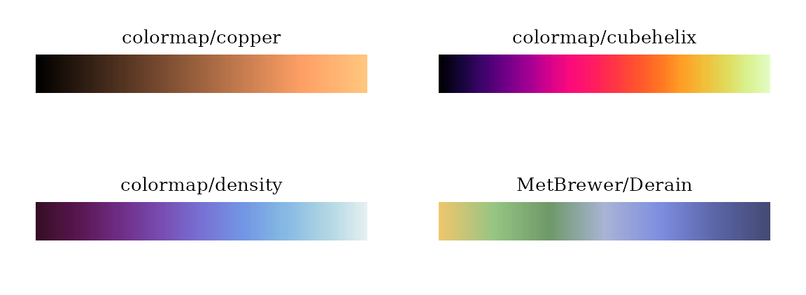
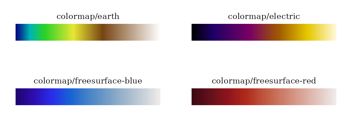
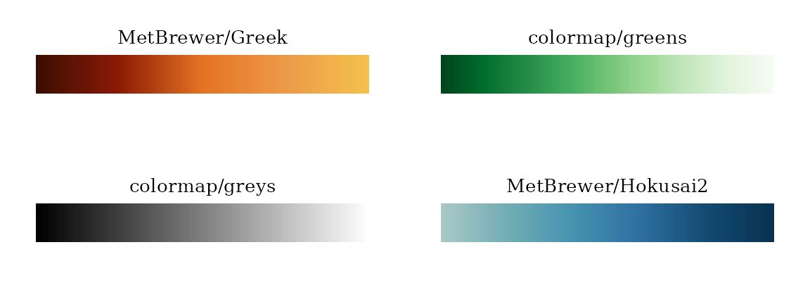
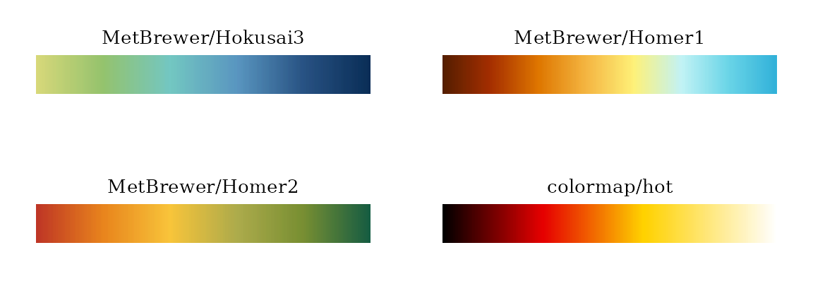
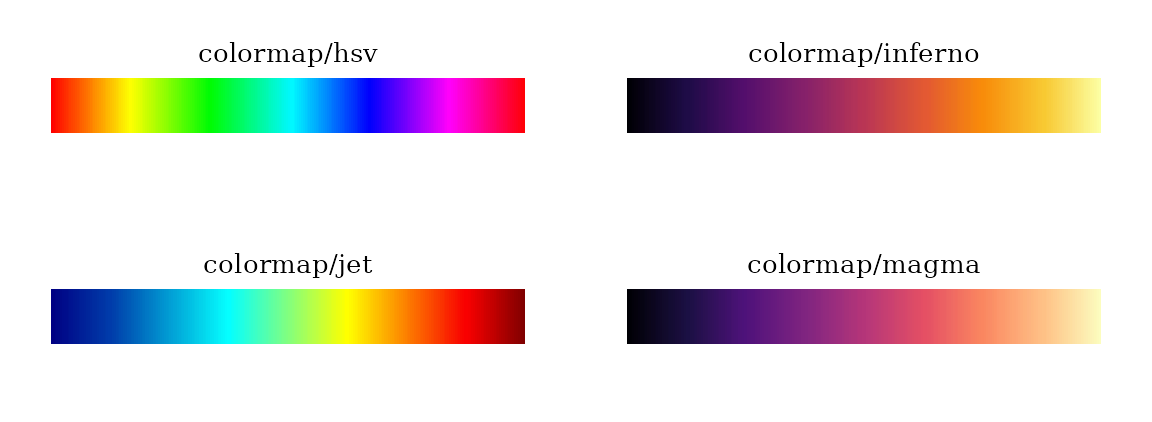
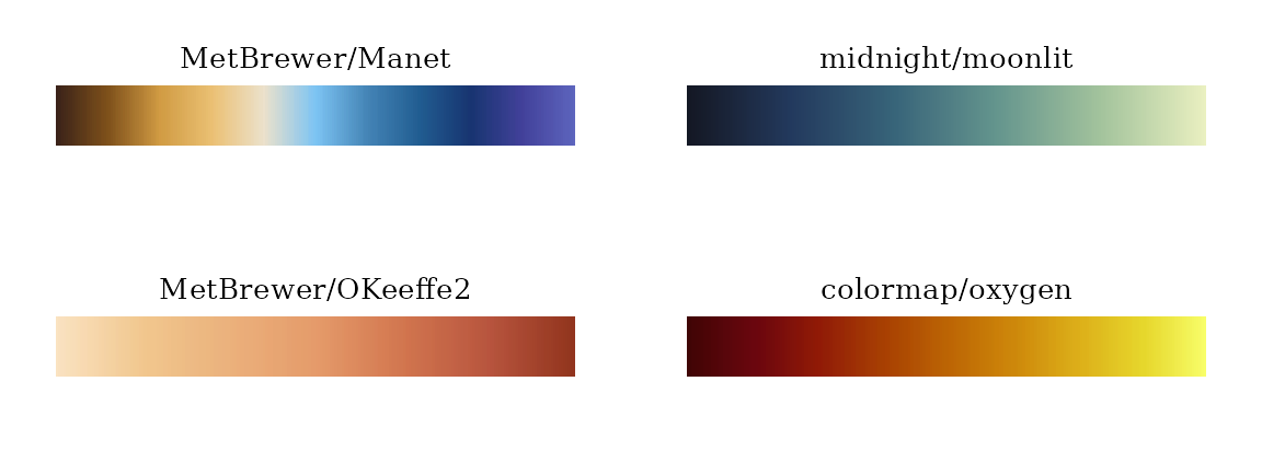
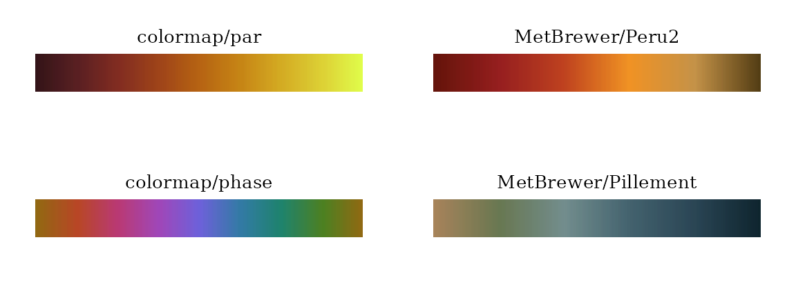
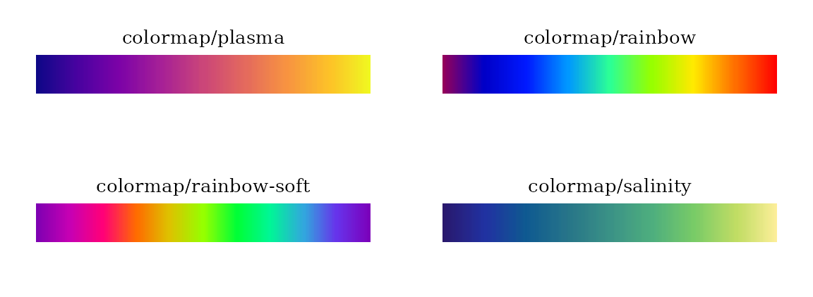
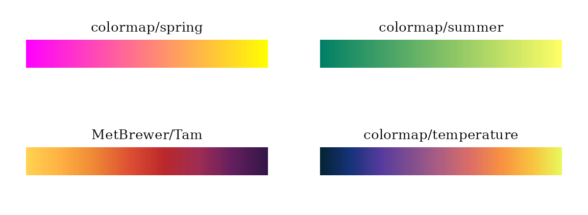
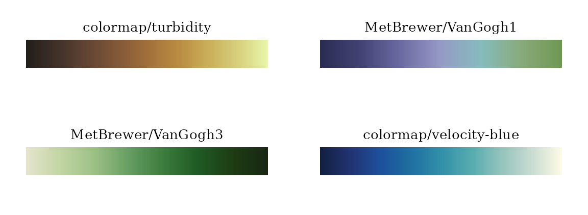
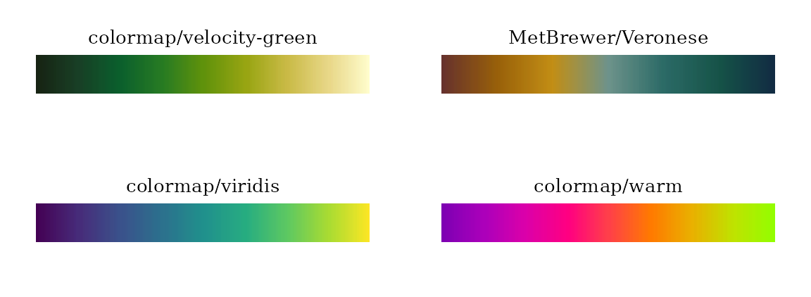
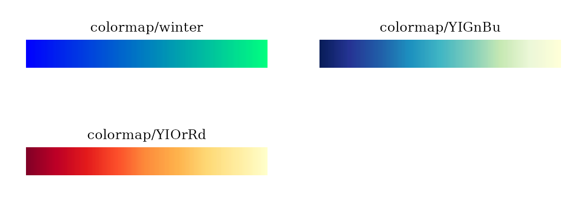
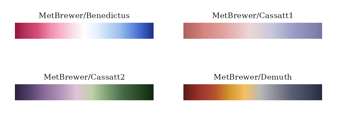
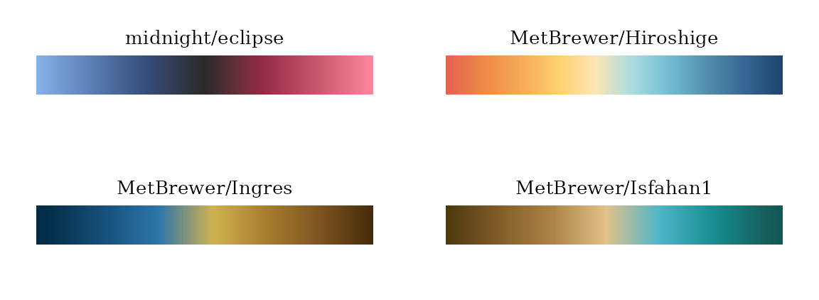
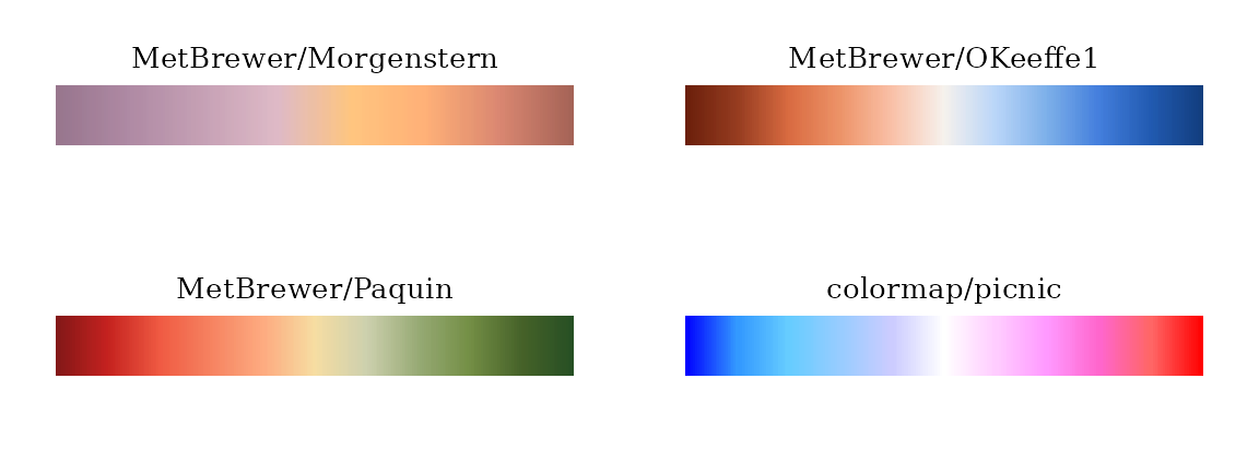
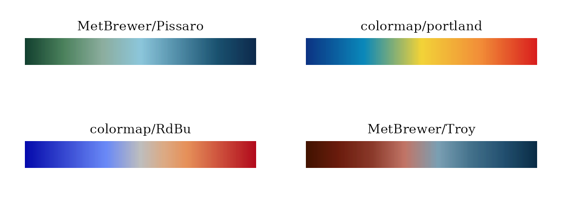
Joint Effect Surface

The S3 method of persp() for “mid” creates surface plots, making it easy to examine the joint effect of two predictors.

par.midr(mar = c(0, 0, 0, 0))
persp(mid$fit, "Wind:Solar.R", theta = 45, phi = 30)

Additional Color Themes

To ensure the visualizations are both accurate and aesthetically pleasing, midnight adds a wide array of color palettes from colormap, DALEX and MetBrewer as well as three original themes.

Qualitative Themes

Sequential Themes

Diverging Themes

Summary

The midnight package combines the computational speed of fastLmMatrix() with the modern API of tidymodels via mid_reg(). When paired with its powerful visualization and color theme systems, it provides a comprehensive toolkit for building, scaling, and interpreting sophisticated models.