interpret() is used to fit a Maximum Interpretation Decomposition (MID) model.
MID models are additive, highly interpretable models composed of functions, each with up to two variables.
Usage
interpret(object, ...)

# Default S3 method
interpret(
  object,
  x,
  y = NULL,
  weights = NULL,
  pred.fun = get.yhat,
  link = NULL,
  k = c(NA, NA),
  type = c(1L, 1L),
  interactions = FALSE,
  terms = NULL,
  singular.ok = FALSE,
  mode = 1L,
  method = NULL,
  lambda = 0,
  kappa = 1e+06,
  na.action = getOption("na.action"),
  verbosity = 1L,
  frames = list(),
  split = "quantile",
  digits = NULL,
  lump = "none",
  others = "others",
  sep = ">",
  max.nelements = 1000000000L,
  nil = 1e-07,
  tol = 1e-07,
  pred.args = list(),
  ...
)

# S3 method for class 'formula'
interpret(
  formula,
  data = NULL,
  model = NULL,
  pred.fun = get.yhat,
  weights = NULL,
  subset = NULL,
  na.action = getOption("na.action"),
  verbosity = 1L,
  mode = 1L,
  drop.unused.levels = FALSE,
  pred.args = list(),
  ...
)
Arguments
- object
a fitted model object to be interpreted.
- ...
optional arguments. For
interpret.formula(), arguments to be passed on tointerpret.default(). Forinterpret.default(),...can include convenient aliases (e.g., "ok" forsingular.ok, "ie" forinteractions) as well as several advanced fitting options (see the "Advanced Fitting Options" section for details).- x
a matrix or data.frame of predictor variables to be used in the fitting process. The response variable should not be included.
- y
an optional vector or matrix of the model predictions or the response variables.
- weights
a numeric vector of sample weights for each observation in
x.- pred.fun
a function to obtain predictions from a fitted model, where the first argument is for the fitted model and the second argument is for new data. The default is
get.yhat().- link
a character string specifying the link function. This can be one of the links from
make.link()(e.g., "log", "logit", "probit", "cauchit"), one of the links fromget.link()(e.g., "log1p", "robit", "scobit", "box-cox"), or a custom object containing at least thelinkfun()andlinkinv()functions.- k
an integer or a vector of two integers specifying the maximum number of sample points for main effects (
k[1]) and interactions (k[2]). If a single integer is provided, it is used for main effects while the value for interactions is automatically determined. AnyNAvalue will also trigger this automatic determination. With non-positive values, all unique data points are used as sample points.- type
a character string, an integer, or a vector of length two specifying the encoding type. Can be integer (
1for linear,0for step) or character ("linear","constant"). If a vector is passed,type[1L]is used for main effects andtype[2L]is used for interactions.- interactions
logical. If
TRUEand iftermsandformulaare not supplied, all interactions for each pair of variables are modeled and calculated.- terms
a character vector of term labels or formula, specifying the set of component functions to be modeled. If not passed,
termsincludes all main effects, and all second-order interactions ifinteractionsisTRUE.- singular.ok
logical. If
FALSE, a singular fit is an error.- mode
an integer specifying the method of calculation. If
modeis1, the centering constraints are treated as penalties for the least squares problem. Ifmodeis2, the constraints are used to reduce the number of free parameters.- method
an integer or a character string specifying the algorithm to solve the core least squares problem. Built-in options include
0or "qr" (column-pivoted QR),1or "unpivoted.qr",2or "llt" (LLT Cholesky),3or "ldlt" (LDLT Cholesky),4or "svd" (singular value decomposition), and5or "eigen" (eigenvalue-eigenvector decomposition). For multi-response targets (matrixy), the computation automatically utilizes base R equivalents or safely falls back to "qr" withstats::.lm.fit(). External custom solvers can also be injected by settingoptions(midr.solver.<method_name> = function(x, y) ...).- lambda
the penalty factor for pseudo smoothing. The default is
0.- kappa
the penalty factor for centering constraints. Used only when
modeis1. The default is1e+6.- na.action
a function or character string specifying the method of
NAhandling. The default is "na.omit".- verbosity
the level of verbosity.
0: fatal,1: warning (default),2: info or3: debug.- frames
a named list of encoding frames ("numeric.frame" or "factor.frame" objects). The encoding frames are used to encode the variable of the corresponding name. If the name begins with "|" or ":", the encoding frame is used only for main effects or interactions, respectively.
- split
a character string specifying the splitting strategy for numeric variables:
"quantile"or"uniform".- digits
an integer. The rounding digits for encoding numeric variables. Used only when
typeis1or"linear".- lump
a character string specifying the lumping strategy for factor variables:
"none","rank","order", or"auto".- others
a character string specifying the others level.
- sep
a character string used to separate levels when merging ordered factors or creating interaction terms.
- max.nelements
an integer specifying the maximum number of elements of the design matrix. Defaults to
1e9.- nil
a threshold for the intercept and coefficients to be treated as zero. The default is
1e-7.- tol
a tolerance for the singular value decomposition. The default is
1e-7.- pred.args
optional parameters other than the fitted model and new data to be passed to
pred.fun().- formula
a symbolic description of the MID model to be fit.
- data
a data.frame, list or environment containing the variables in
formula. If not found in data, the variables are taken fromenvironment(formula).- model
a fitted model object to be interpreted.
- subset
an optional vector specifying a subset of observations to be used in the fitting process.
- drop.unused.levels
logical. If
TRUE, unused levels of factors will be dropped.
Value
interpret() returns an object of class "mid". This is a list with the following components:
- weights
a numeric vector of the sample weights.
- call
the matched call.
- terms
the
terms.objectused.- link
a "link-glm" or "link-midr" object containing the link function.
- intercept
the intercept.
- encoders
a list of variable encoders.
- main.effects
a list of data frames representing the main effects.
- interactions
a list of data frames representing the interactions.
- ratio
the ratio of the sum of squared error between the target model predictions and the fitted MID values, to the sum of squared deviations of the target model predictions.
- linear.predictors
a numeric vector of the linear predictors.
- fitted.values
a numeric vector of the fitted values.
- residuals
a numeric vector of the working residuals.
- na.action
information about the special handling of
NAs.
If a matrix is provided for y, interpret() returns a "midrib" and "mids" object.
Details
Maximum Interpretation Decomposition (MID) is a functional decomposition framework designed to serve as a faithful surrogate for complex, black-box models. It deconstructs a target prediction function \(f(\mathbf{X})\) into a set of highly interpretable components:
$$f(\mathbf{X}) = g_\emptyset + \sum_{j} g_j(X_j) + \sum_{j<k} g_{jk}(X_j, X_k) + g_D(\mathbf{X})$$
where \(g_\emptyset\) is the intercept, \(g_j(X_j)\) represents the main effect of feature \(j\), \(g_{jk}(X_j, X_k)\) represents the second-order interaction between features \(j\) and \(k\), and \(g_D(\mathbf{X})\) is the residual.
The components \(g_j\) and \(g_{jk}\) are modeled as a linear expansion of basis functions, resulting in piecewise linear or piecewise constant functions. The estimation is performed by minimizing a penalized squared residual objective over a representative dataset:
$$\text{minimize } \mathbf{E}[g_D(\mathbf{X})^2] + \lambda R(g;\mathbf{X})$$
where \(\lambda \ge 0\) is a regularization parameter that controls the smoothness of the components by penalizing the second-order differences of adjacent coefficients (a discrete roughness penalty).
To ensure the uniqueness and identifiability of the decomposition, MID imposes the centering constraints: for any feature \(j\), \(\mathbf{E}[g_j(X_j)] = 0\); and for any feature pair \((j, k)\), \(\mathbf{E}[g_{jk}(X_j, X_k) \mid X_j = x_j] = 0\) for all \(x_j\) and \(\mathbf{E}[g_{jk}(X_j, X_k) \mid X_k = x_k] = 0\) for all \(x_k\). In cases where the least-squares solution is still not unique due to collinearity, an additional probability-weighted minimum-norm constraint is applied to the coefficients to ensure a stable and unique solution.
Advanced Fitting Options
The ... argument can be used to pass several advanced fitting options:
- fit.intercept
logical. If
TRUE, the intercept term is fitted as part of the least squares problem. IfFALSE(default), it is calculated as the weighted mean of the response.- interpolation
a character string specifying the method for interpolating inestimable coefficients (betas) that arise from sparse data regions. Can be "iterative" for an iterative smoothing process, "direct" for solving a linear system, or "none" to disable interpolation.
- max.niterations
an integer specifying the maximum number of iterations for the "iterative" interpolation method.
- save.memory
an integer (0, 1, or 2) specifying the memory-saving level. Higher values reduce memory usage at the cost of increased computation time.
- weighted.norm
logical. If
TRUE, the columns of the design matrix are normalized by the square root of their weighted sum. This is required to ensure the minimum-norm least squares solution obtained by appropriate methods (i.e.,4or5) offastLmPure()is the minimum-norm solution in a weighted sense.- weighted.encoding
logical. If
TRUE, sample weights are used during the encoding process (e.g., for calculating quantiles to determine knots).
References
Asashiba R, Kozuma R, Iwasawa H (2025). “midr: Learning from Black-Box Models by Maximum Interpretation Decomposition.” 2506.08338, https://arxiv.org/abs/2506.08338.
Examples
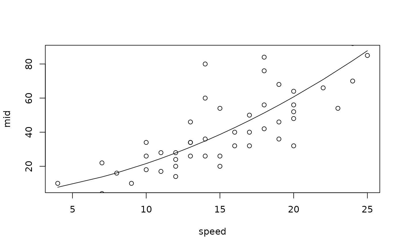
# Fit a MID model as a surrogate for another model
data(cars, package = "datasets")
model <- lm(dist ~ I(speed^2) + speed, cars)
mid <- interpret(dist ~ speed, cars, model)
plot(mid, "speed", intercept = TRUE)
points(cars)
 # Fit a MID model as a standalone predictive model
data(airquality, package = "datasets")
mid <- interpret(Ozone ~ .^2, data = airquality, lambda = .5)
#> 'model' not passed: response variable in 'data' is used
plot(mid, "Wind")
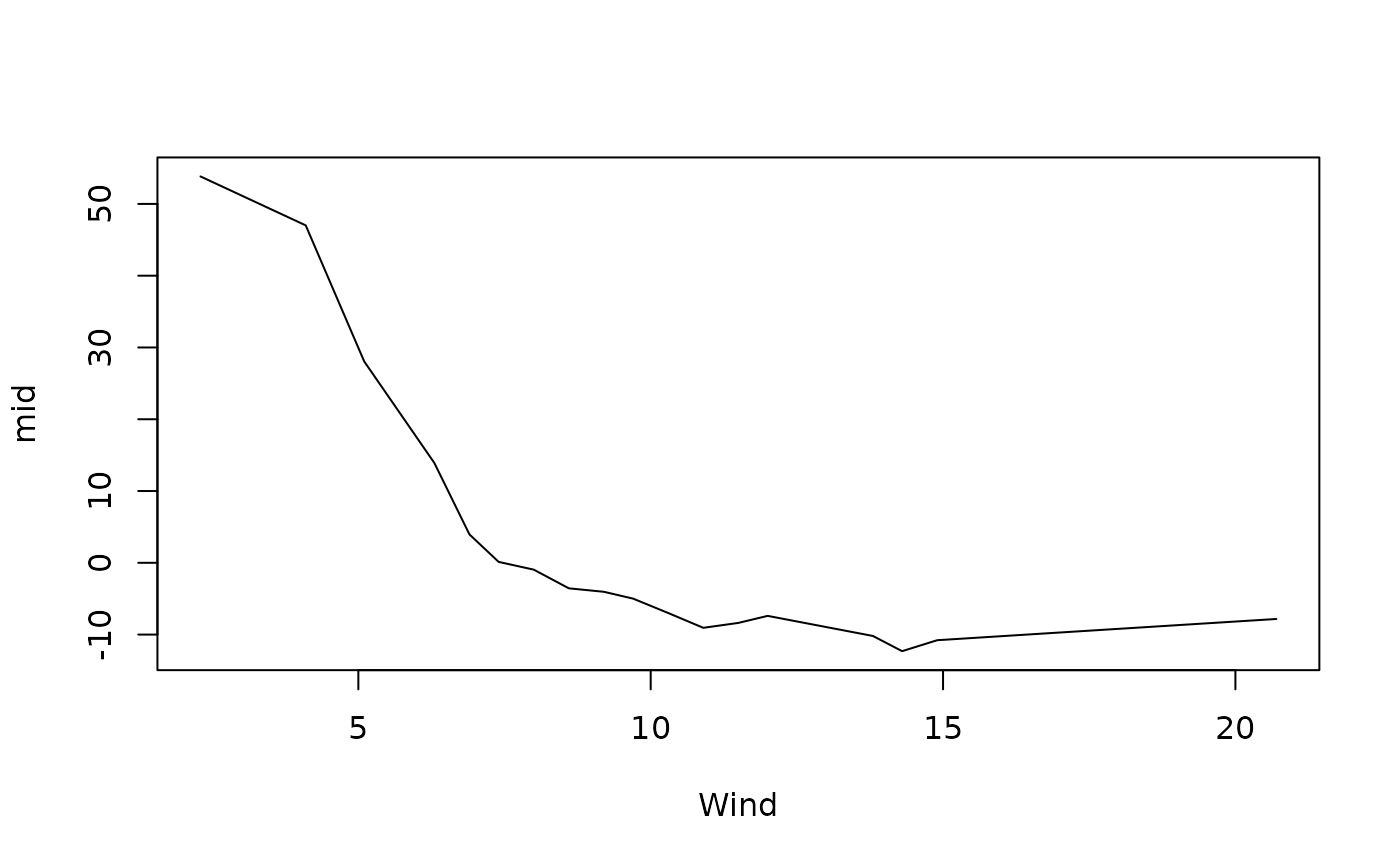
# Fit a MID model as a standalone predictive model
data(airquality, package = "datasets")
mid <- interpret(Ozone ~ .^2, data = airquality, lambda = .5)
#> 'model' not passed: response variable in 'data' is used
plot(mid, "Wind")
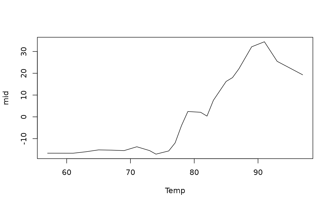
 plot(mid, "Temp")
 plot(mid, "Wind:Temp", main.effects = TRUE)
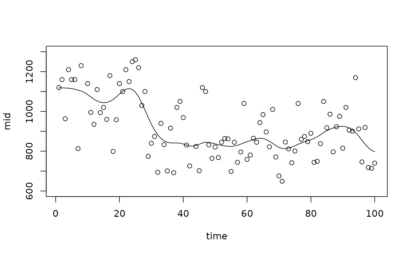
 data(Nile, package = "datasets")
nile <- data.frame(time = 1:length(Nile), flow = as.numeric(Nile))
# A flexible fit with many knots
mid <- interpret(flow ~ time, data = nile, k = 100L)
#> 'model' not passed: response variable in 'data' is used
plot(mid, "time", intercept = TRUE, limits = c(600L, 1300L))
points(x = 1L:100L, y = Nile)
data(Nile, package = "datasets")
nile <- data.frame(time = 1:length(Nile), flow = as.numeric(Nile))
# A flexible fit with many knots
mid <- interpret(flow ~ time, data = nile, k = 100L)
#> 'model' not passed: response variable in 'data' is used
plot(mid, "time", intercept = TRUE, limits = c(600L, 1300L))
points(x = 1L:100L, y = Nile)
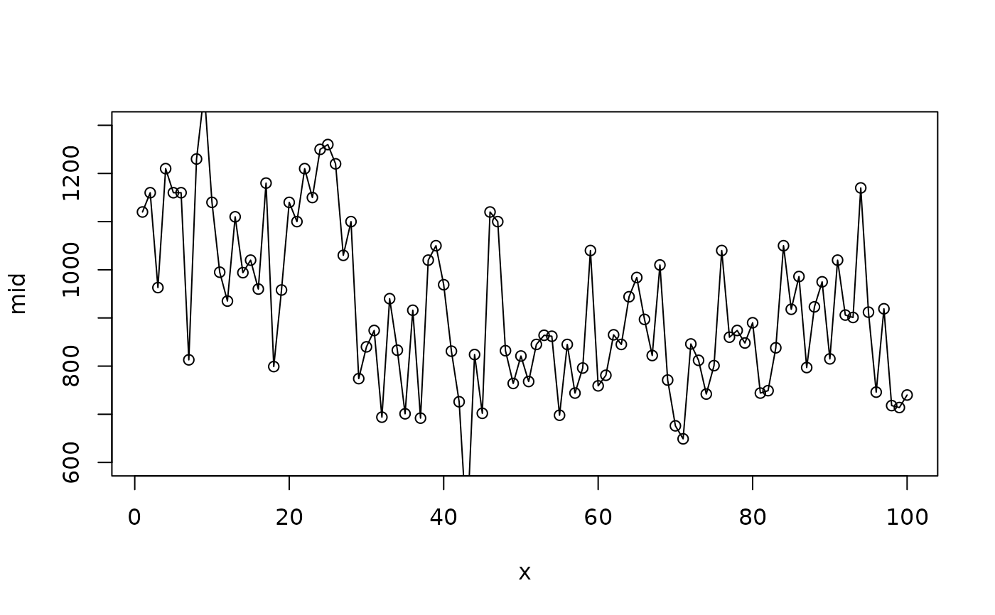
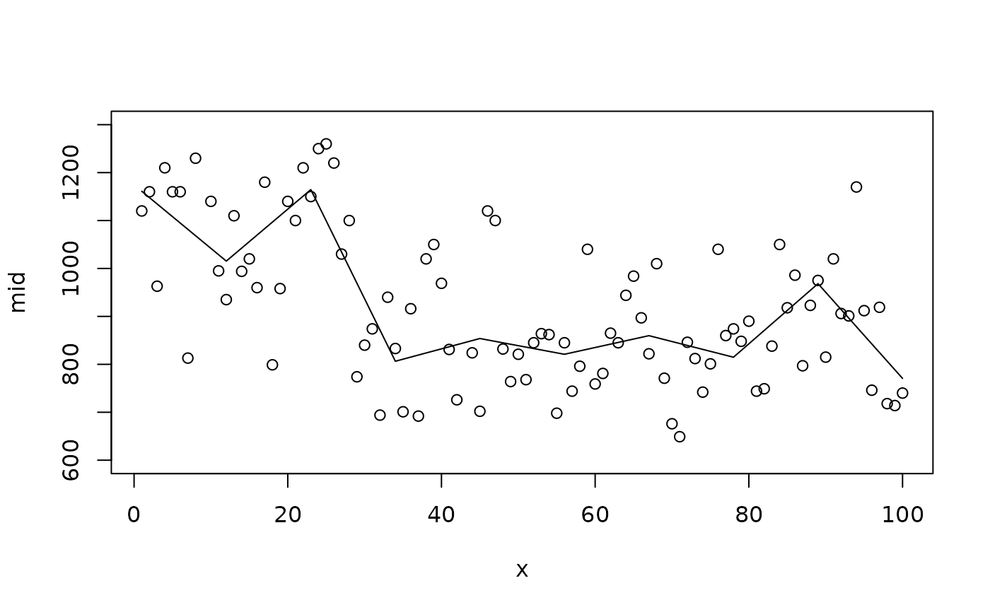
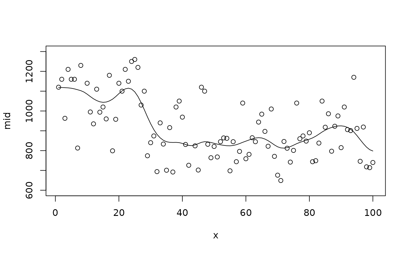
 # A smoother fit with fewer knots
mid <- interpret(flow ~ time, data = nile, k = 10L)
#> 'model' not passed: response variable in 'data' is used
plot(mid, "time", intercept = TRUE, limits = c(600L, 1300L))
points(x = 1L:100L, y = Nile)
# A smoother fit with fewer knots
mid <- interpret(flow ~ time, data = nile, k = 10L)
#> 'model' not passed: response variable in 'data' is used
plot(mid, "time", intercept = TRUE, limits = c(600L, 1300L))
points(x = 1L:100L, y = Nile)
 # A pseudo-smoothed fit using a penalty
mid <- interpret(flow ~ time, data = nile, k = 100L, lambda = 100L)
#> 'model' not passed: response variable in 'data' is used
plot(mid, "time", intercept = TRUE, limits = c(600L, 1300L))
points(x = 1L:100L, y = Nile)
# A pseudo-smoothed fit using a penalty
mid <- interpret(flow ~ time, data = nile, k = 100L, lambda = 100L)
#> 'model' not passed: response variable in 'data' is used
plot(mid, "time", intercept = TRUE, limits = c(600L, 1300L))
points(x = 1L:100L, y = Nile)