This article presents some examples of the interpretation of
regression models using midr.
# load required packages
library(midr)
library(ggplot2)
library(gridExtra)
library(patchwork)
library(Metrics)
theme_set(theme_midr())
Regression Task
We use a benchmark regression task, originally described in Friedman
(1991) and Breiman (1996), and implemented in the mlbench
package. The dataset has 10 independent predictor variables
each uniformly distributed on the interval
,
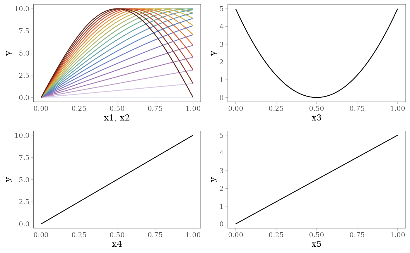
and the response variable
, generated according to the following formula with disturbance term
.
The following plots show the effect of each predictor variable on the response. For and , the interaction effect is shown by the colored lines: the effect of depends on the value of (pale purple for 0 and dark red for 1) and vice versa.
# benchmark regression task
library(mlbench)
set.seed(42)
train  <- as.data.frame(mlbench.friedman1(n = 500L))
test   <- as.data.frame(mlbench.friedman1(n = 500L))
mtrain <- as.data.frame(mlbench.friedman1(n = 2500L))[, -11L]
For each model type, we fit a regression model using the
train data of 500 observations and an interpretative MID
surrogate of the target model using the mtrain data of 2500
observations without the response variable. We then evaluate the
predictive accuracy of the target model and the interpretative accuracy
of the MID surrogate based on the RMSE between the test and
model prediction or the two predictions, respectively.
# define utility functions for the following chunks
effect_plots <- function(object) {
  mid.plots(object, terms = paste("x", 1:6, sep = "."))
}

interaction_plot <- function(object) {
  ggmid(object, "x.1:x.2", main.effects = TRUE, theme = "sunset") +
    ggtitle("interaction effect")
}

ice_theme <- color.theme("mako")
ice_plot <- function(object, data = train[1:200, ]) {
  ggmid(mid.conditional(object, "x.1", data = data),
        var.color = x.2, type = "centered", theme = ice_theme) +
    ggtitle("conditional expectation")
}

importance_plot <- function(object) {
  ggmid(mid.importance(object), "heatmap") +
    ggtitle("feature importance")
}

eval_plot <- function(model, mid, data = test, ...) {
  pred <- get.yhat(model, data, ...)
  pred_mid <- get.yhat(mid, data)
  actual <- test$y
  rmse_vs_test <- rmse(pred, actual)
  rmse_vs_mid <-  rmse(pred, pred_mid)
  ggplot() + scale_color_theme("highlight?accent='steelblue'") +
    geom_point(aes(x = pred, y = actual, col = "vs test")) +
    geom_point(aes(x = pred, y = pred_mid, col = "vs mid")) +
    geom_abline(slope = 1, intercept = 0, col = "black", lty = 2) +
    labs(x = "model-prediction", y = "mid-prediction / test") +
    annotate(
      "text", family = "serif", size = 3,
      x = min(pred) + diff(range(pred)) / 8,
      y = max(actual) - diff(range(actual) / 8),
      label = sprintf("RMSE\nvs test: %.3f\nvs mid: %.3f",
                      rmse_vs_test, rmse_vs_mid)
    ) + ggtitle("prediction / representation accuracy")
}
ml <- midlist()
Additive Models
Linear Model
model <- lm(y ~ ., train)
coef(model)
#> (Intercept)         x.1         x.2         x.3         x.4         x.5
#>   0.1302510   6.8458545   6.8892805  -0.4403955  10.3264576   4.6735425
#>         x.6         x.7         x.8         x.9        x.10
#>   0.5837944   0.2030152  -0.6272202  -0.1722106   0.3453933
mid <- interpret(y ~ .^2, mtrain, model)
print(mid)
#>
#> Call:
#> interpret(formula = y ~ .^2, data = mtrain, model = model)
#>
#> Model Class: lm
#>
#> Intercept: 14.319
#>
#> Main Effects:
#> 10 main effect terms
#>
#> Interactions:
#> 45 interaction terms
#>
#> Uninterpreted Variation Ratio: 0
grid.arrange(grobs = effect_plots(mid), nrow = 2L)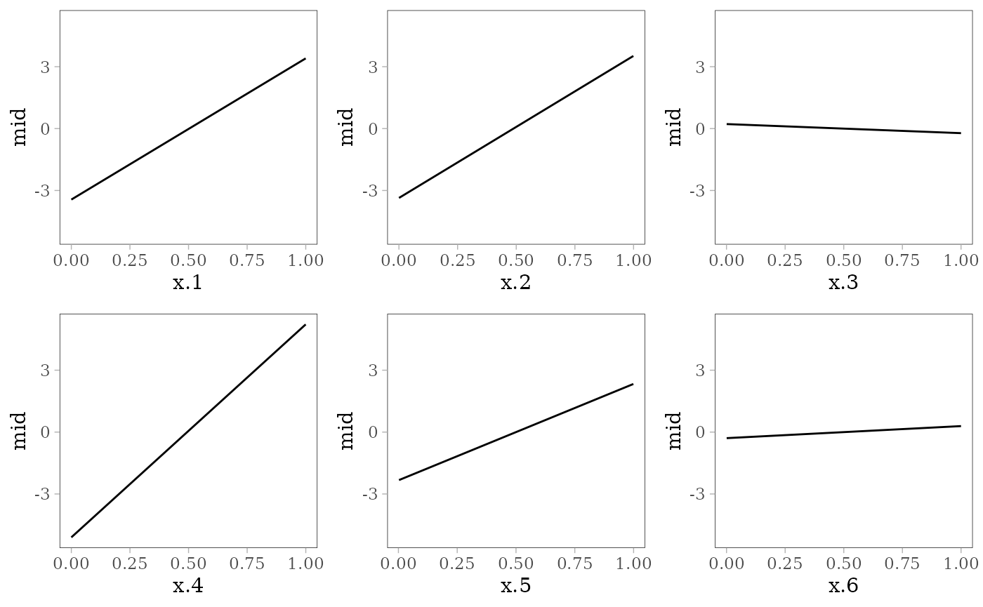
grid.arrange(interaction_plot(mid), importance_plot(mid),
             ice_plot(mid), eval_plot(model, mid), nrow = 2)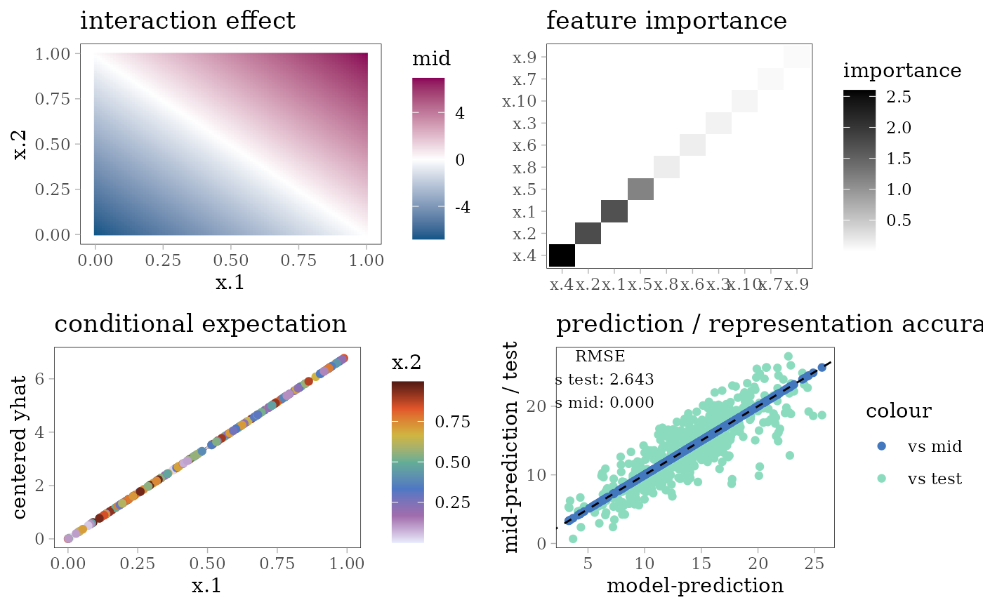
ml$lm <- midRegularized GLM
library(glmnet)
model <- glmnet(x = as.matrix(train[, -11]), y = train[, 11])
# prediction with arbitrarily chosen lambda
mid <- interpret(y ~ .^2, mtrain[, -11], model,
                 pred.args = list(s = model$lambda[9]))
print(mid)
#>
#> Call:
#> interpret(formula = y ~ .^2, data = mtrain[, -11], model = model,
#>  pred.args = list(s = model$lambda[9]))
#>
#> Model Class: elnet, glmnet
#>
#> Intercept: 14.374
#>
#> Main Effects:
#> 10 main effect terms
#>
#> Interactions:
#> 45 interaction terms
#>
#> Uninterpreted Variation Ratio: 0
grid.arrange(grobs = effect_plots(mid), nrow = 2L)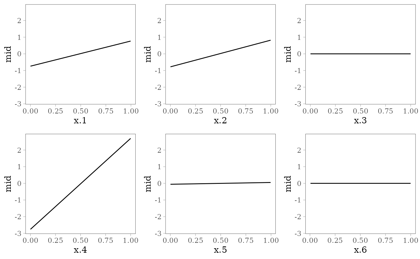
evp <- eval_plot(model, mid, data = test[, -11],
                       s = model$lambda[9])
grid.arrange(interaction_plot(mid), importance_plot(mid),
             ice_plot(mid), evp, nrow = 2)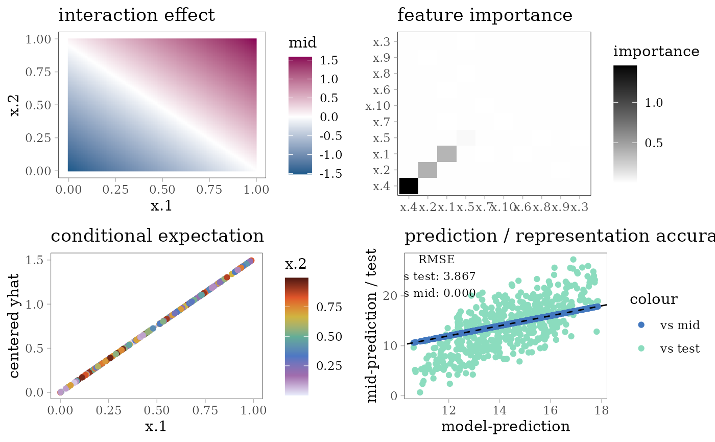
Generalized Additive Model
library(gam)
model <- gam(y ~ s(x.1) + s(x.2) + s(x.3) + s(x.4) + s(x.5) +
             s(x.6) + s(x.7) + s(x.8) + s(x.9) + s(x.10),
             family = gaussian, data = train)
mid <- interpret(y ~ .^2, mtrain, model)
print(mid)
#>
#> Call:
#> interpret(formula = y ~ .^2, data = mtrain, model = model)
#>
#> Model Class: Gam, glm, lm
#>
#> Intercept: 14.323
#>
#> Main Effects:
#> 10 main effect terms
#>
#> Interactions:
#> 45 interaction terms
#>
#> Uninterpreted Variation Ratio: 3.9583e-07
grid.arrange(grobs = effect_plots(mid), nrow = 2L)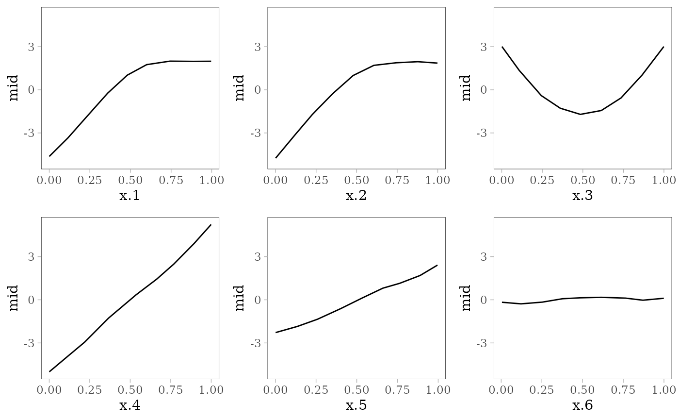
grid.arrange(interaction_plot(mid), importance_plot(mid),
             ice_plot(mid), eval_plot(model, mid), nrow = 2)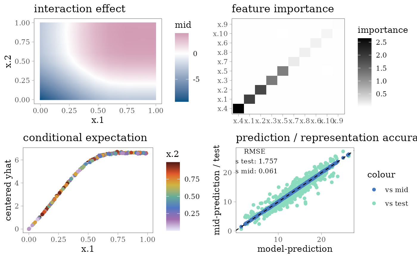
ml$gam <- midMultivariate Adaptive Regression Spline
library(earth)
model <- earth(y ~ ., degree = 2, data = train)
mid <- interpret(y ~ .^2, mtrain, model)
print(mid)
#>
#> Call:
#> interpret(formula = y ~ .^2, data = mtrain, model = model)
#>
#> Model Class: earth
#>
#> Intercept: 14.182
#>
#> Main Effects:
#> 10 main effect terms
#>
#> Interactions:
#> 45 interaction terms
#>
#> Uninterpreted Variation Ratio: 0.00051402
grid.arrange(grobs = effect_plots(mid), nrow = 2L)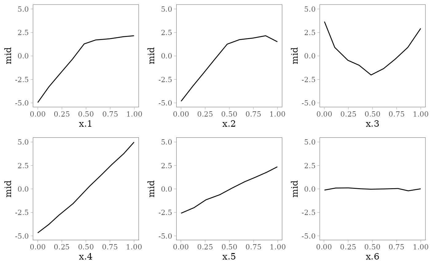
grid.arrange(interaction_plot(mid), importance_plot(mid),
             ice_plot(mid), eval_plot(model, mid), nrow = 2)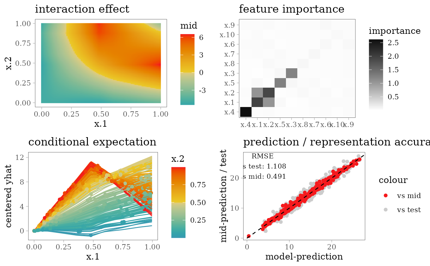
ml$mars <- midNeural Network
Single Hidden Layer Network
library(nnet)
set.seed(42)
model <- nnet(y ~ ., train, size = 5, linout = TRUE, maxit = 1e3, trace = FALSE)
mid <- interpret(y ~ .^2, mtrain, model)
print(mid)
#>
#> Call:
#> interpret(formula = y ~ .^2, data = mtrain, model = model)
#>
#> Model Class: nnet.formula, nnet
#>
#> Intercept: 14.195
#>
#> Main Effects:
#> 10 main effect terms
#>
#> Interactions:
#> 45 interaction terms
#>
#> Uninterpreted Variation Ratio: 0.00281
grid.arrange(grobs = effect_plots(mid), nrow = 2L)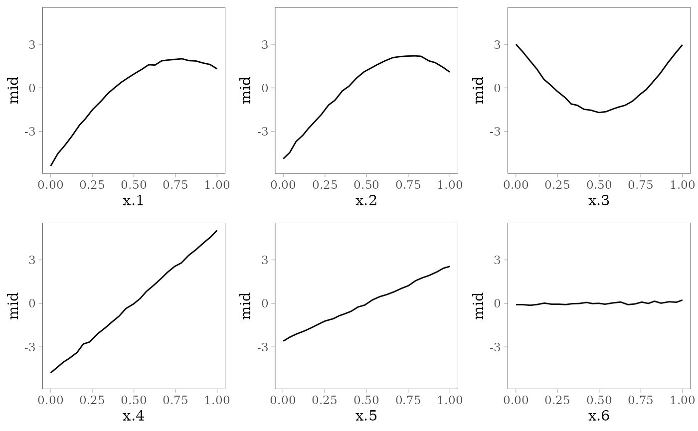
grid.arrange(interaction_plot(mid), importance_plot(mid),
             ice_plot(mid), eval_plot(model, mid), nrow = 2)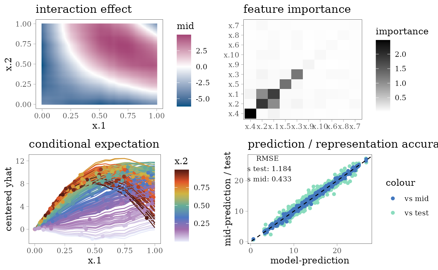
ml$nnet <- midSupport Vector Machine
RBF Kernel SVM
library(e1071)
#>
#> Attaching package: 'e1071'
#> The following object is masked from 'package:ggplot2':
#>
#>     element
model <- svm(y ~ ., train, kernel = "radial")
mid <- interpret(y ~ .^2, mtrain, model)
print(mid)
#>
#> Call:
#> interpret(formula = y ~ .^2, data = mtrain, model = model)
#>
#> Model Class: svm.formula, svm
#>
#> Intercept: 14.32
#>
#> Main Effects:
#> 10 main effect terms
#>
#> Interactions:
#> 45 interaction terms
#>
#> Uninterpreted Variation Ratio: 0.0075534
grid.arrange(grobs = effect_plots(mid), nrow = 2L)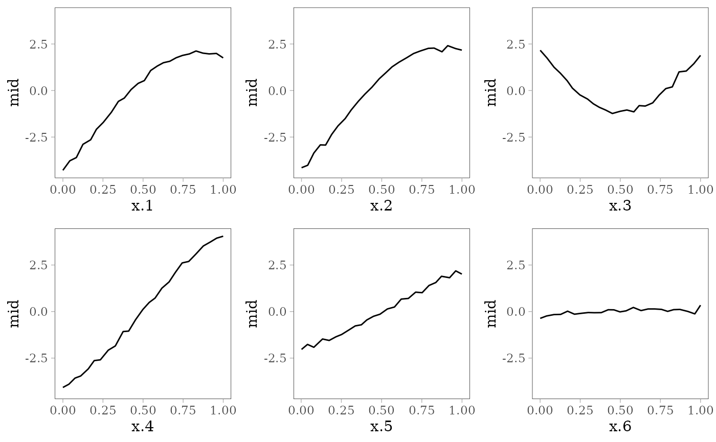
grid.arrange(interaction_plot(mid), importance_plot(mid),
             ice_plot(mid), eval_plot(model, mid), nrow = 2)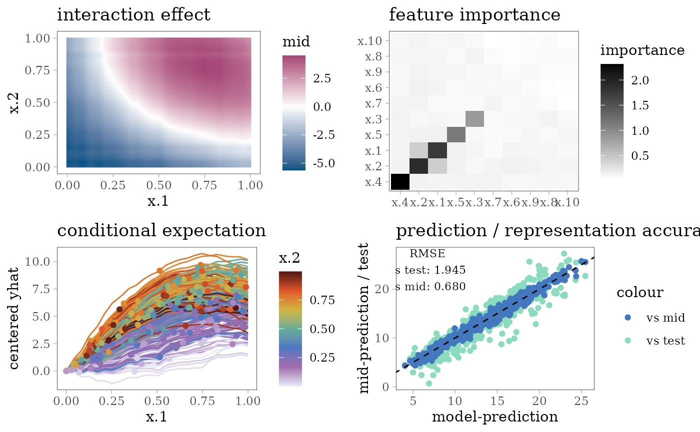
ml$svm <- midTree Based Models
Gradient Boosting Trees
library(xgboost)
params <- list(eta = .1, subsample = .7, max_depth = 5)
set.seed(42)
model <- xgboost(as.matrix(train[, -11]), train[, 11], nrounds = 100,
                 params = params, verbose = 0)
#> Warning in throw_err_or_depr_msg("Parameter(s) have been removed from this
#> function: ", : Parameter(s) have been removed from this function: params. This
#> warning will become an error in a future version.
#> Warning in throw_err_or_depr_msg("Passed unrecognized parameters: ",
#> paste(head(names_unrecognized), : Passed unrecognized parameters: verbose. This
#> warning will become an error in a future version.
mid <- interpret(y ~ .^2, as.matrix(mtrain), model)
print(mid)
#>
#> Call:
#> interpret(formula = y ~ .^2, data = as.matrix(mtrain), model = model)
#>
#> Model Class: xgboost, xgb.Booster
#>
#> Intercept: 14.307
#>
#> Main Effects:
#> 10 main effect terms
#>
#> Interactions:
#> 45 interaction terms
#>
#> Uninterpreted Variation Ratio: 0.030268
grid.arrange(grobs = effect_plots(mid), nrow = 2L)
evp <- eval_plot(model, mid, as.matrix(test[, -11]))
grid.arrange(interaction_plot(mid), importance_plot(mid),
             ice_plot(mid), evp, nrow = 2)
ml$xgb <- midRandom Forest
library(ranger)
set.seed(42)
model <- ranger(y ~ ., train, mtry = 5)
mid <- interpret(y ~ .^2, mtrain, model)
print(mid)
#>
#> Call:
#> interpret(formula = y ~ .^2, data = mtrain, model = model)
#>
#> Model Class: ranger
#>
#> Intercept: 14.27
#>
#> Main Effects:
#> 10 main effect terms
#>
#> Interactions:
#> 45 interaction terms
#>
#> Uninterpreted Variation Ratio: 0.0075659
grid.arrange(grobs = effect_plots(mid), nrow = 2L)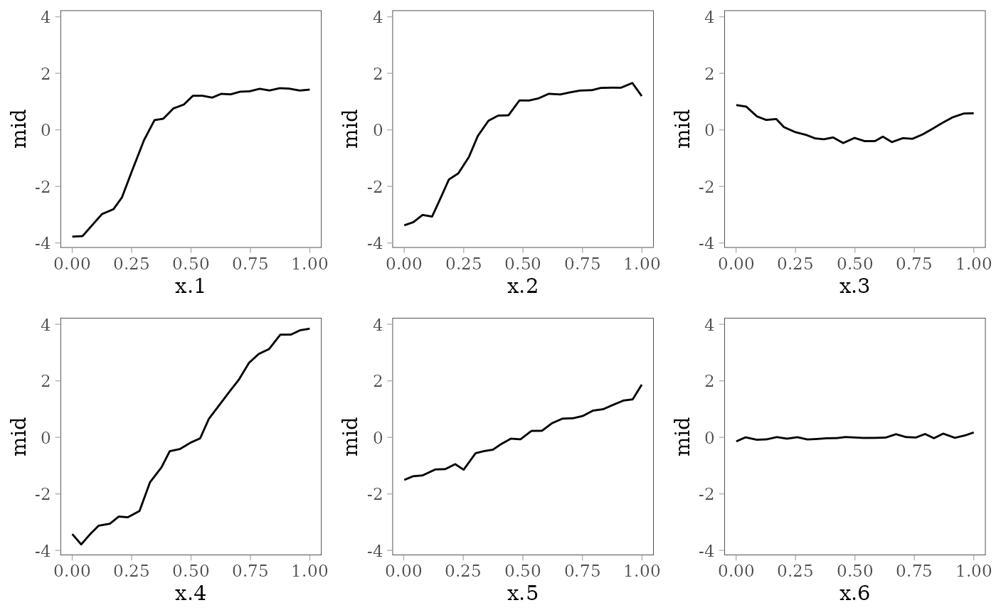
grid.arrange(interaction_plot(mid), importance_plot(mid),
             ice_plot(mid), eval_plot(model, mid), nrow = 2)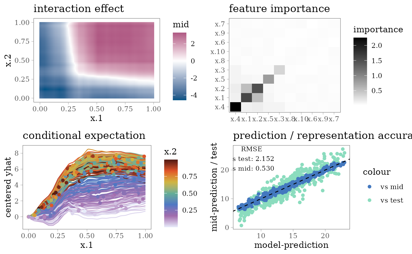
ml$rf <- midDecision Tree
library(rpart)
model <- rpart(y ~ ., train)
# create encoding frames for CART
frm <- cbind(model$frame, labels(model, collapse = FALSE))
print(t(frm[frm$var != "<leaf>", c("var", "ltemp")]))
#>       1          2        5         11         22         3          7
#> var   "x.4"      "x.1"    "x.2"     "x.4"      "x.5"      "x.2"      "x.1"
#> ltemp "< 0.5579" "< 0.21" "< 0.311" "< 0.2953" "< 0.5849" "< 0.2653" "< 0.3184"
#>       14         15         31         62
#> var   "x.4"      "x.5"      "x.4"      "x.2"
#> ltemp "< 0.8843" "< 0.2486" "< 0.8413" "< 0.4782"
frames <- lapply(mtrain, range)
frames$x.1 <- c(frames$x.1, .2100, .3184)
frames$x.2 <- c(frames$x.2, .3110, .2653, .4782)
frames$x.4 <- c(frames$x.4, .5579, .2953, .8843, .8413)
frames$x.5 <- c(frames$x.5, .5849, .2486)
mid <- interpret(y ~ .^2, mtrain, model, type = 0, frames = frames)
print(mid)
#>
#> Call:
#> interpret(formula = y ~ .^2, data = mtrain, model = model, type = 0,
#>  frames = frames)
#>
#> Model Class: rpart
#>
#> Intercept: 14.264
#>
#> Main Effects:
#> 10 main effect terms
#>
#> Interactions:
#> 45 interaction terms
#>
#> Uninterpreted Variation Ratio: 0.031256
grid.arrange(grobs = effect_plots(mid), nrow = 2L)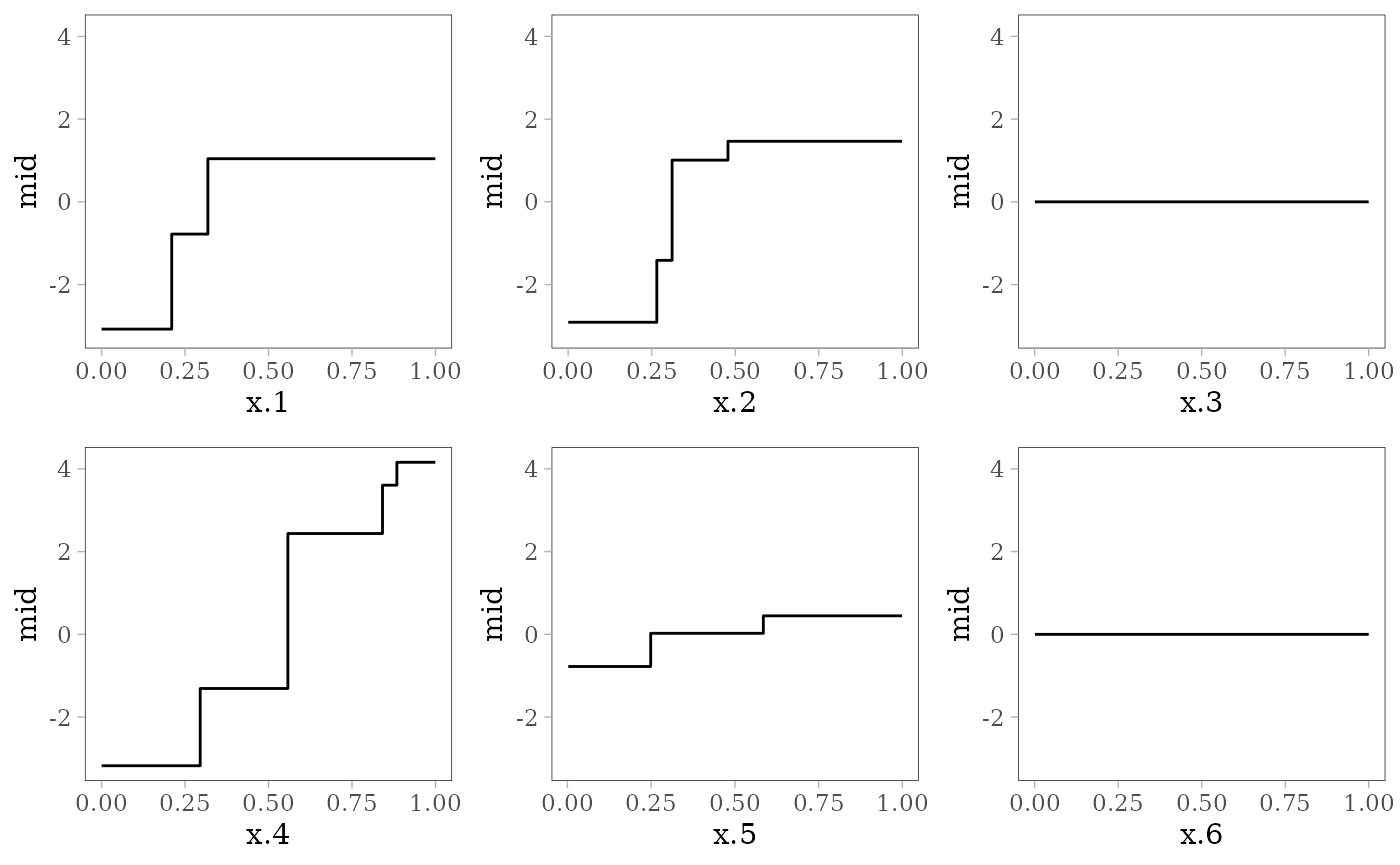
grid.arrange(interaction_plot(mid), importance_plot(mid),
             ice_plot(mid), eval_plot(model, mid), nrow = 2)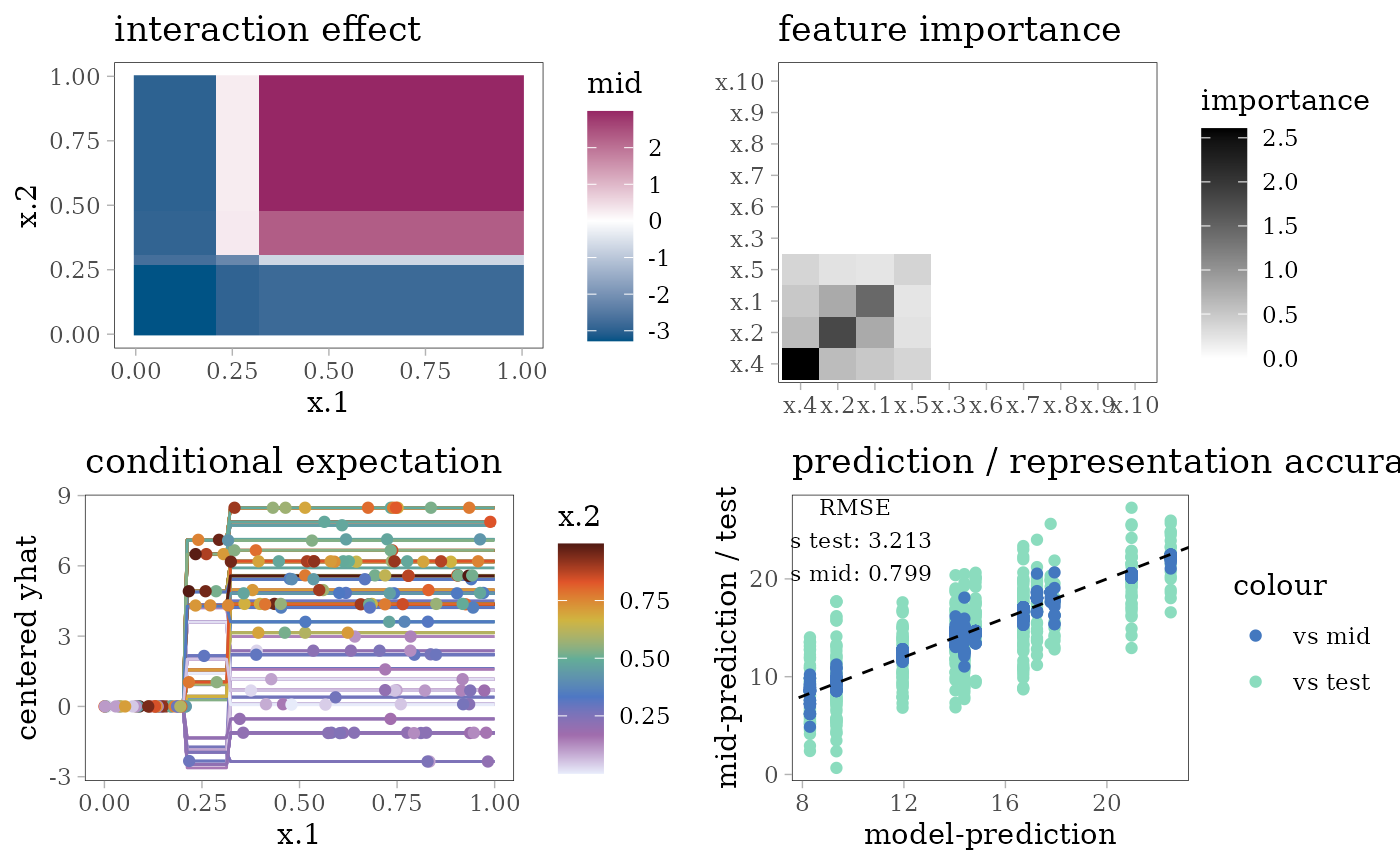
ml$tree <- midOther Modes
Predictive MID
model <- mid <- interpret(y ~ .^2, train, lambda = .2)
#> 'model' not passed: response variable in 'data' is used
pred <- pred_mid <- predict(mid, test)
print(mid)
#>
#> Call:
#> interpret(formula = y ~ .^2, data = train, lambda = 0.2)
#>
#> Intercept: 14.417
#>
#> Main Effects:
#> 10 main effect terms
#>
#> Interactions:
#> 45 interaction terms
#>
#> Uninterpreted Variation Ratio: 0.03179
grid.arrange(grobs = effect_plots(mid), nrow = 2L)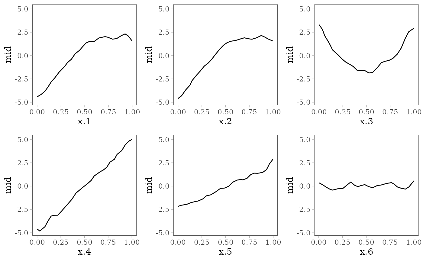
grid.arrange(interaction_plot(mid), importance_plot(mid),
             ice_plot(mid), eval_plot(model, mid), nrow = 2)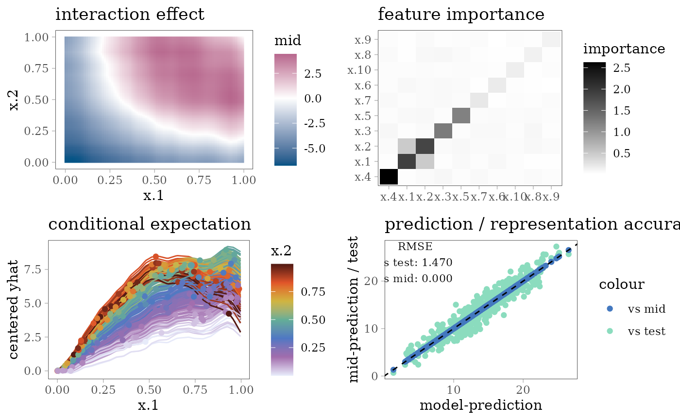
Compare Multiple Models
p1 <- ggmid(ml[1:4], "x.1") + theme(legend.position = "none")
p2 <- ggmid(ml[1:4], "x.3") + theme(legend.position = "none")
p3 <- ggmid(ml[1:4], "x.4")
p4 <- ggmid(ml[5:8], "x.1") + theme(legend.position = "none")
p5 <- ggmid(ml[5:8], "x.3") + theme(legend.position = "none")
p6 <- ggmid(ml[5:8], "x.4")
(p1+ p2 + p3) / (p4 + p5 + p6)
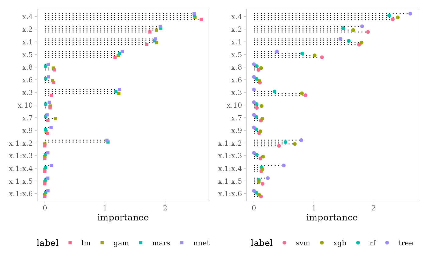
impl <- mid.importance(ml)
p1 <- ggmid(impl[1:4], type = "dotchart", pch = 15) +
  theme(legend.position = "bottom")
p2 <- ggmid(impl[5:8], type = "dotchart", terms = mid.terms(impl)) +
  theme(legend.position = "bottom")
p1 + p2