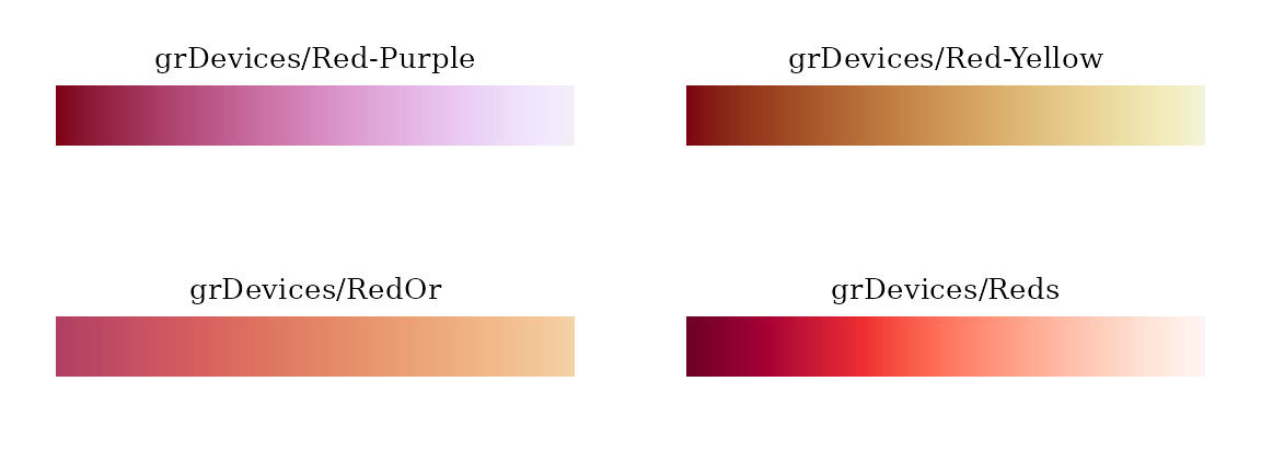
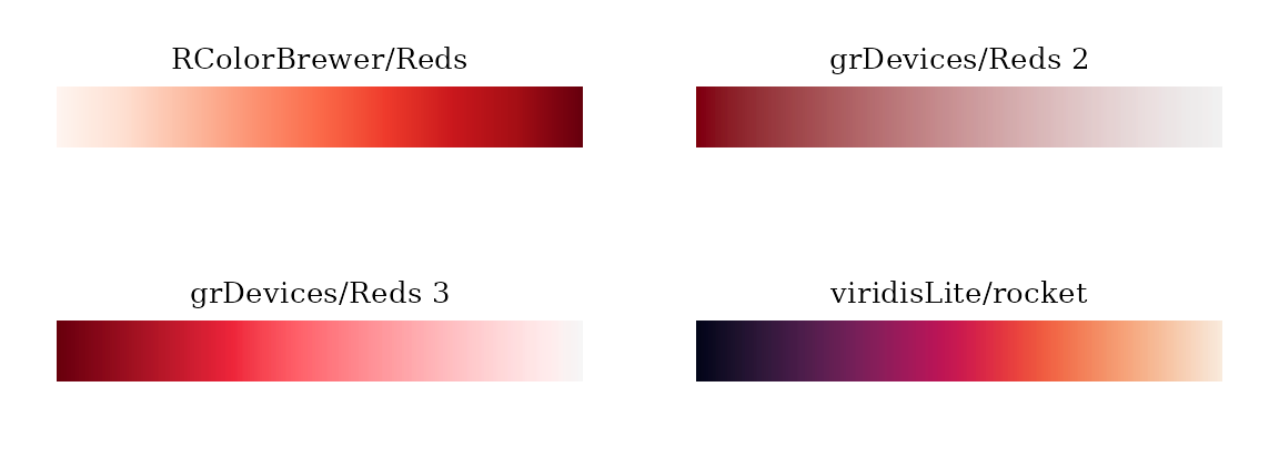
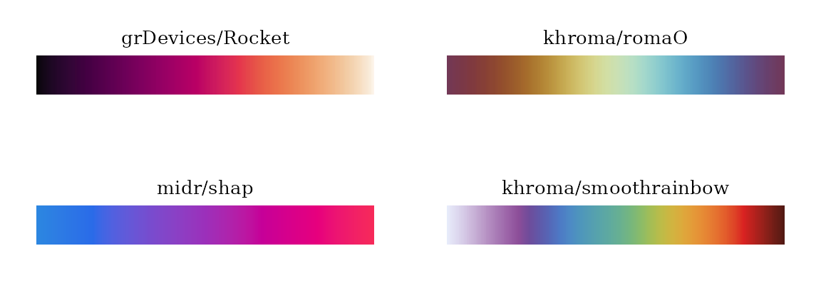
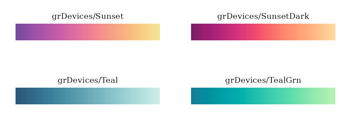
Color themes
The “color.theme” object provides two color-generating functions:
palette() and ramp(). The
palette() function accepts an integer
and returns a vector of
discrete colors. It is primarily intended for
qualitative themes, where distinct colors are used to
represent categorical data. The ramp() function accepts a
numeric vector
with values in the
interval and returns a vector of corresponding colors. It maps numeric
values onto a continuous color gradient, making it suitable for
sequential and diverging themes.
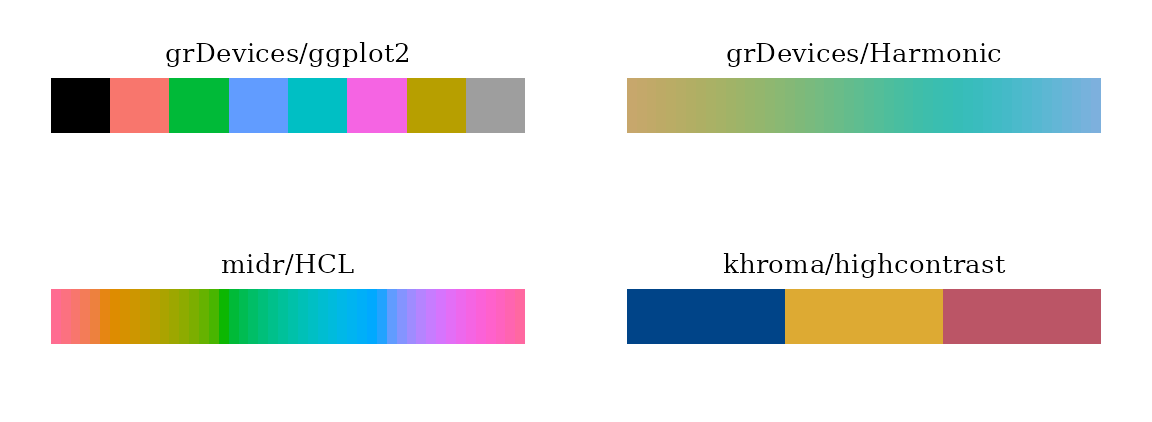
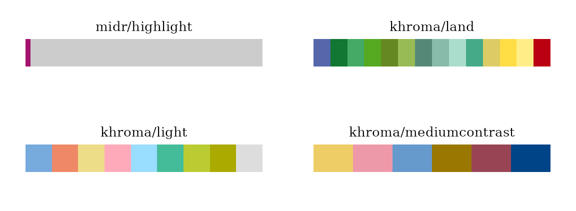
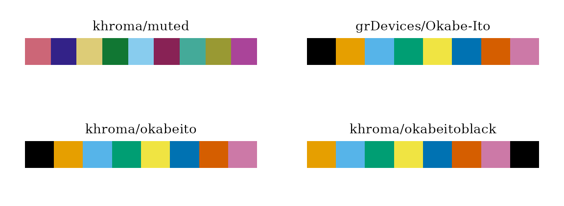
Pre-defined themes
You can get a pre-defined “color.theme” object by providing a theme
name to the color.theme() function.
library(midr)
library(ggplot2)
library(gridExtra)
# diverging color theme "nightfall" (package:khroma)
nightfall <- color.theme("nightfall")
print(nightfall)
#> Diverging Color Theme : "nightfall"
nightfall$palette(5)
#> [1] "#125A56" "#60BCE9" "#ECEADA" "#FD9A44" "#A01813"
#> attr(,"missing")
#> [1] "#FFFFFF"
nightfall$ramp(c(0.00, 0.25, 0.50, 0.75, 1.00))
#> [1] "#125955" "#5FBBE9" "#EBEAD9" "#FD9944" "#9F1813"
# sequential color theme "viridis" (package:viridisLite)
viridis <- color.theme("viridis")
print(viridis)
#> Sequential Color Theme : "viridis"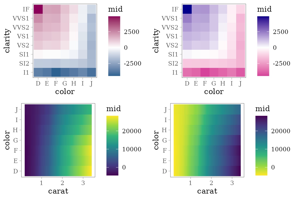
nightfall$ramp(c(0.00, 0.25, 0.50, 0.75, 1.00))
#> [1] "#125955" "#5FBBE9" "#EBEAD9" "#FD9944" "#9F1813"
viridis$ramp(c(0.00, 0.25, 0.50, 0.75, 1.00))
#> [1] "#404486" "#2E6C8D" "#21908C" "#2EB37B" "#79D151"
You can modify themes by reversing the color order or changing the theme type (e.g., from sequential to qualitative). These changes can be applied in two ways:
-
Using Arguments : provide the appropriate argument
to the function, such as
reverse = TRUEortype = "qualitative". -
Using Suffixes : for convenience, you can append a
suffix directly to the theme’s name.
_rto reverse the theme,@q(or longer, such as@qual) to make the theme qualitative (@dfor diverging,@sfor sequential).
plot(color.theme("nightfall", reverse = TRUE),
     text = "khroma/nightfall_r")
plot(color.theme("nightfall", type = "qualitative"),
     text = "khroma/nightfall@qual")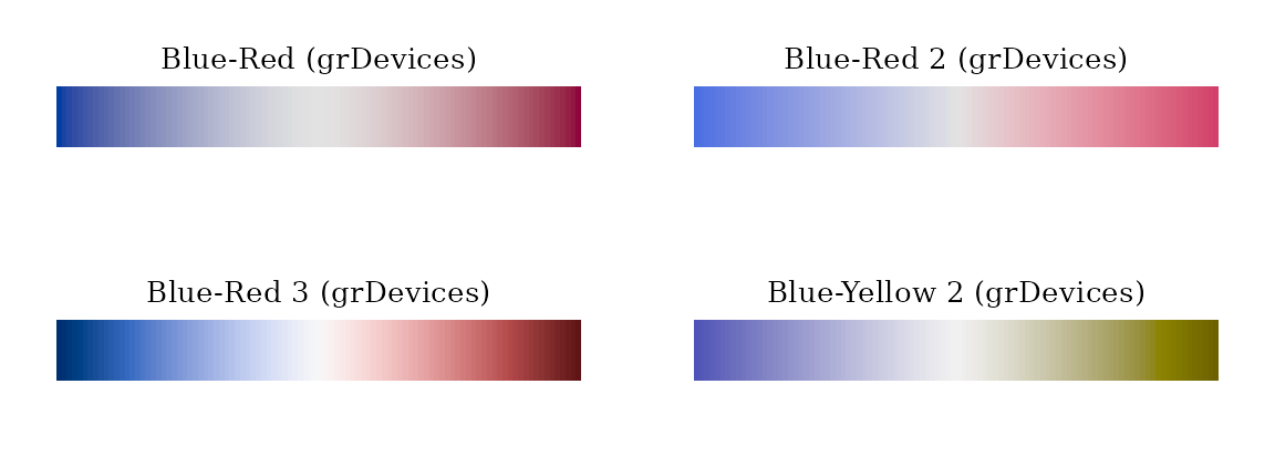
plot(color.theme("viridis_r",),
     text = "viridisLite/viridis_r")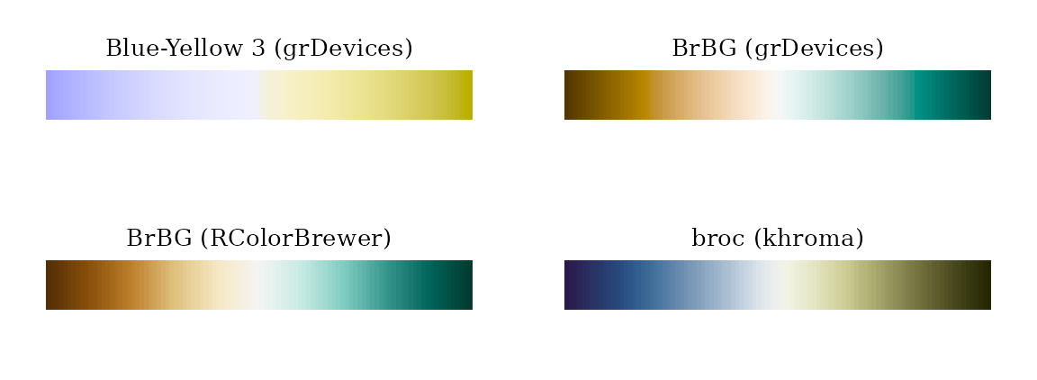
plot(color.theme("viridis@qual"),
     text = "viridisLite/viridis@qual")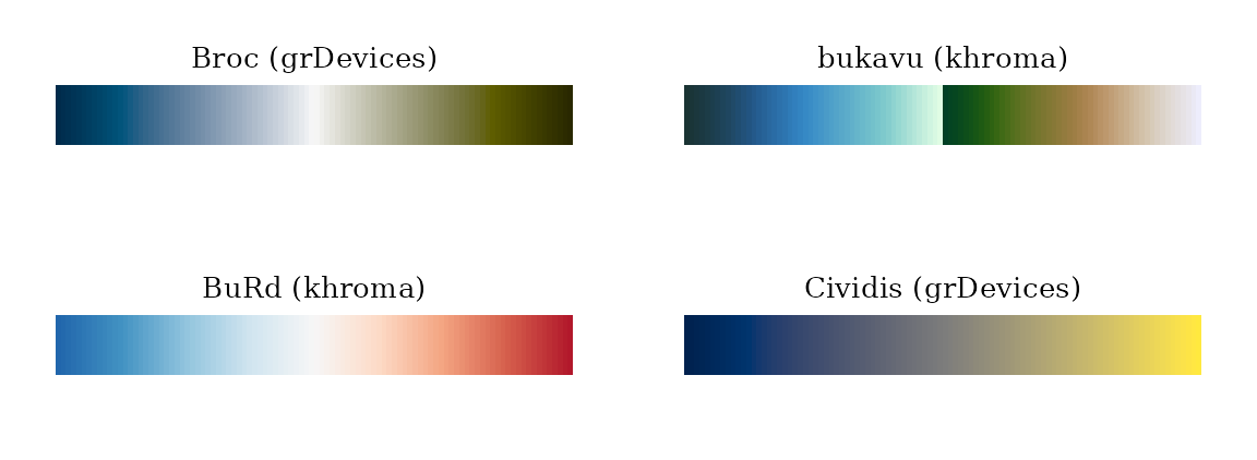
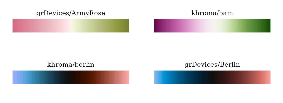
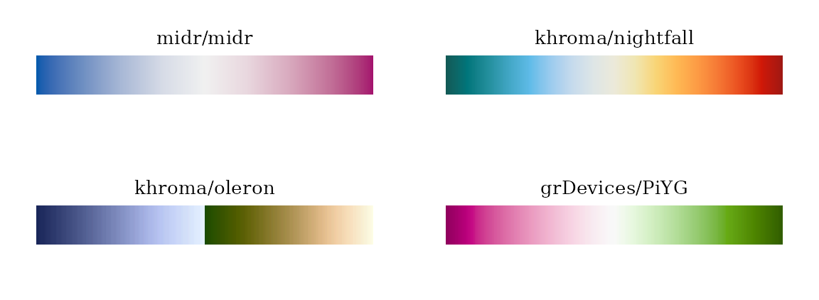
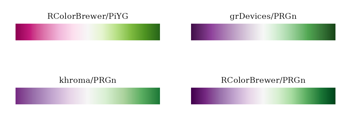
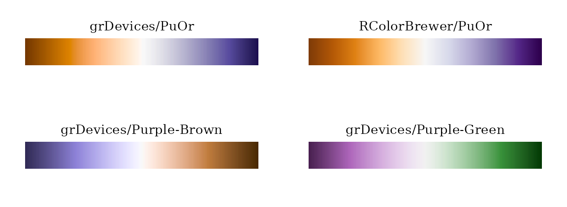
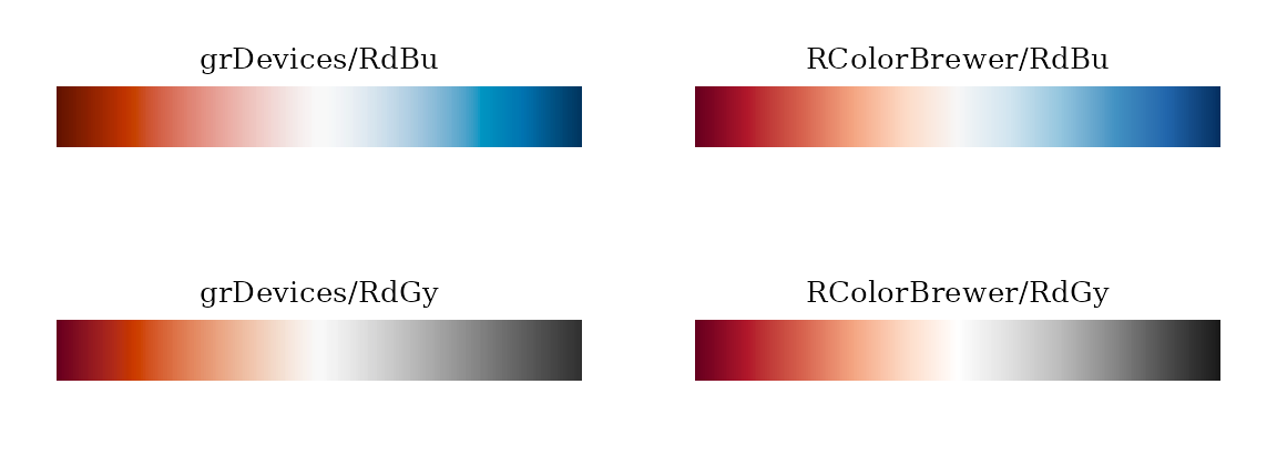
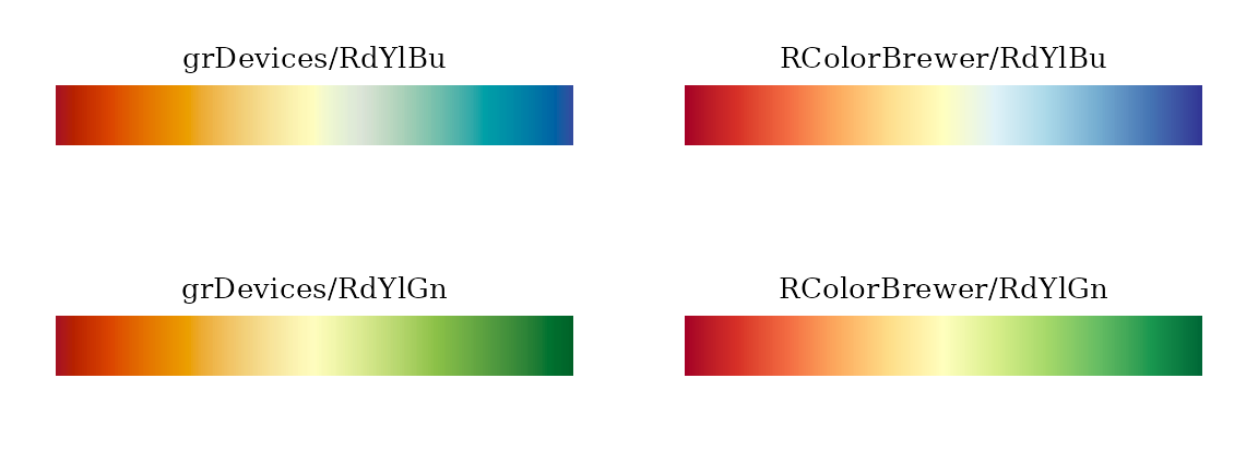
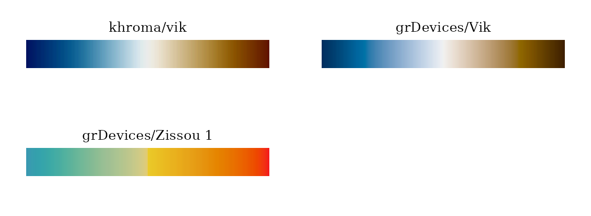
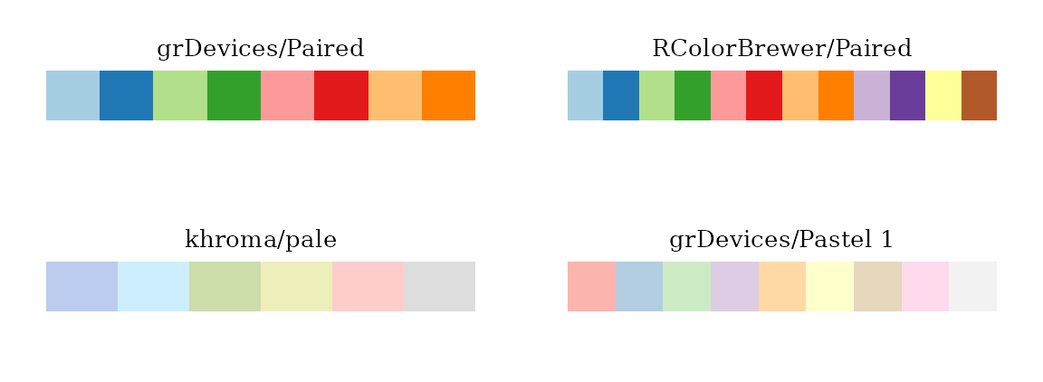
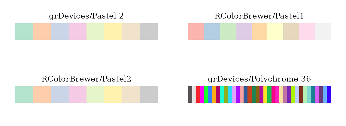
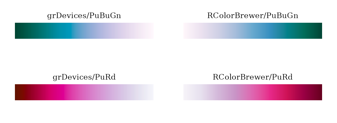
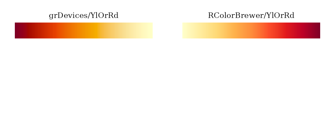
When multiple packages provide a theme with the same name (e.g., “Paired”), you must specify which one to use. You can do this in two ways:
-
Using Argument : provide the package name to the
sourceargument (e.g.,source = "grDevices"). -
Using Prefix : append a prefix to the theme name
with the package name and a forward slash (e.g.,
"RColorBrewer/Paired").
# qualitative color theme "Paired" (package:grDevices)
paired <- color.theme("Paired", source = "grDevices")
plot(paired, text = "grDevices/Paired")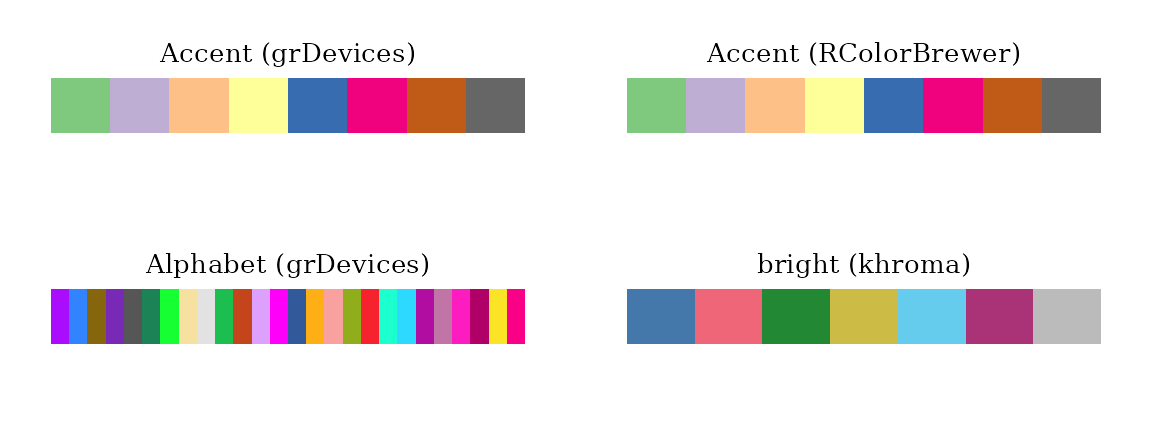
# qualitative color theme "Paired" (package:RColorBrewer)
paired2 <- color.theme("RColorBrewer/Paired")
plot(paired2, text = "RColorBrewer/Paired")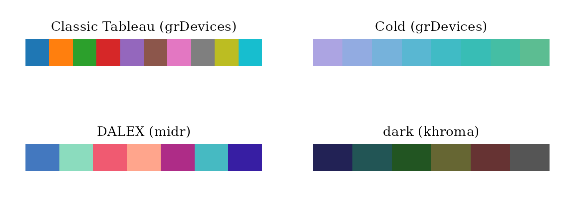
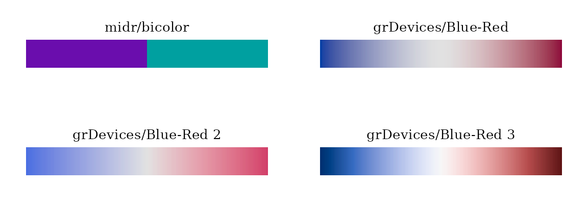
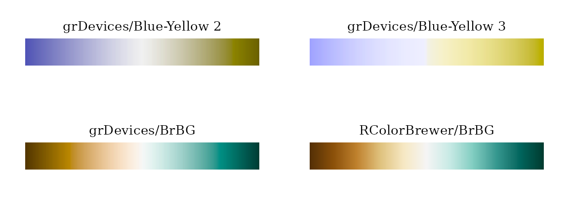
Custom themes
Alternatively, you can create a new “color.theme” object by passing a
custom color vector or function to the first argument of
color.theme().
# create new color theme using a color vector
mytheme <- color.theme(
  c("#003f5c", "#7a5195", "#ef5675", "#ffa600"),
  type = "sequential", name = "mytheme"
)
print(mytheme)
#> Sequential Color Theme : "mytheme"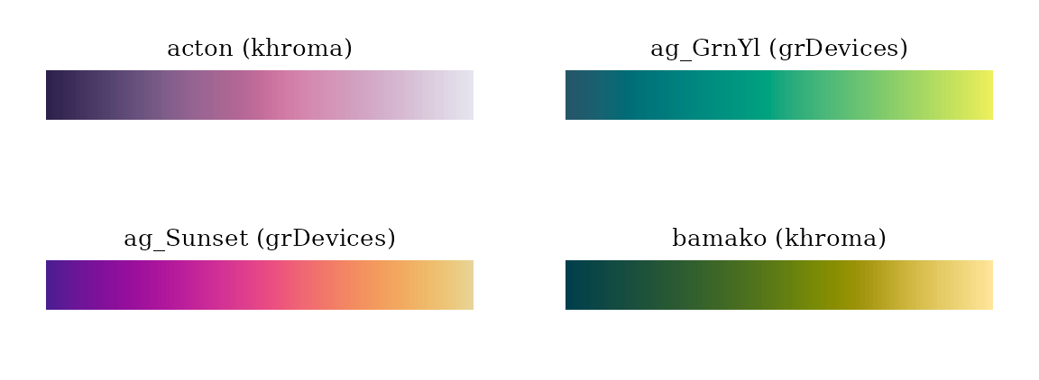
mytheme$palette(5)
#> [1] "#003F5B" "#614D86" "#B85485" "#F46C63" "#FFA500"
mytheme$ramp(c(0.00, 0.25, 0.50, 0.75, 1.00))
#> [1] "#003F5B" "#614D86" "#B85485" "#F46C63" "#FFA500"
# create new color theme using a color function
rainbow <- color.theme(grDevices::rainbow,
                       name = "rainbow", source = "grDevices")
print(rainbow)
#> Sequential Color Theme : "rainbow"
rainbow$palette(5)
#> [1] "#FF0000" "#CCFF00" "#00FF66" "#0066FF" "#CC00FF"
rainbow$ramp(c(0.00, 0.25, 0.50, 0.75, 1.00))
#> [1] "#FF0000" "#81FF00" "#00FFFB" "#7B00FF" "#FF0006"
You can register a custom theme to call it by name later in you
current R session. To do so, use the set.color.theme()
function.
set.color.theme(mytheme, name = "mytheme", source = "custom")
color.theme("mytheme_r@div")
#> Diverging Color Theme : "mytheme"
color.theme("custom/mytheme@q")
#> Qualitative Color Theme : "mytheme"
Using themes in midr
The color appearance of visualizations created with
midr can be easily customized by passing a
“color.theme” object or a pre-defined color theme name (see below) to
ggmid() or plot().
set.seed(42)
dataset <- diamonds[sample(nrow(diamonds), 5000L), ]
mid <- interpret(price ~ (carat + color + clarity + cut) ^ 2, dataset)
#> 'model' not passed: response variable in 'data' is used
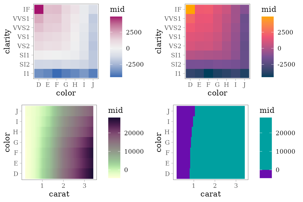
grid.arrange(
ggmid(mid, "color:clarity", main.effect = TRUE),
ggmid(mid, "color:clarity", main.effect = TRUE, theme = mytheme),
ggmid(mid, "carat:color", main.effect = TRUE, theme = "tokyo_r"),
ggmid(mid, "carat:color", main.effect = TRUE, theme = "bicolor")
)
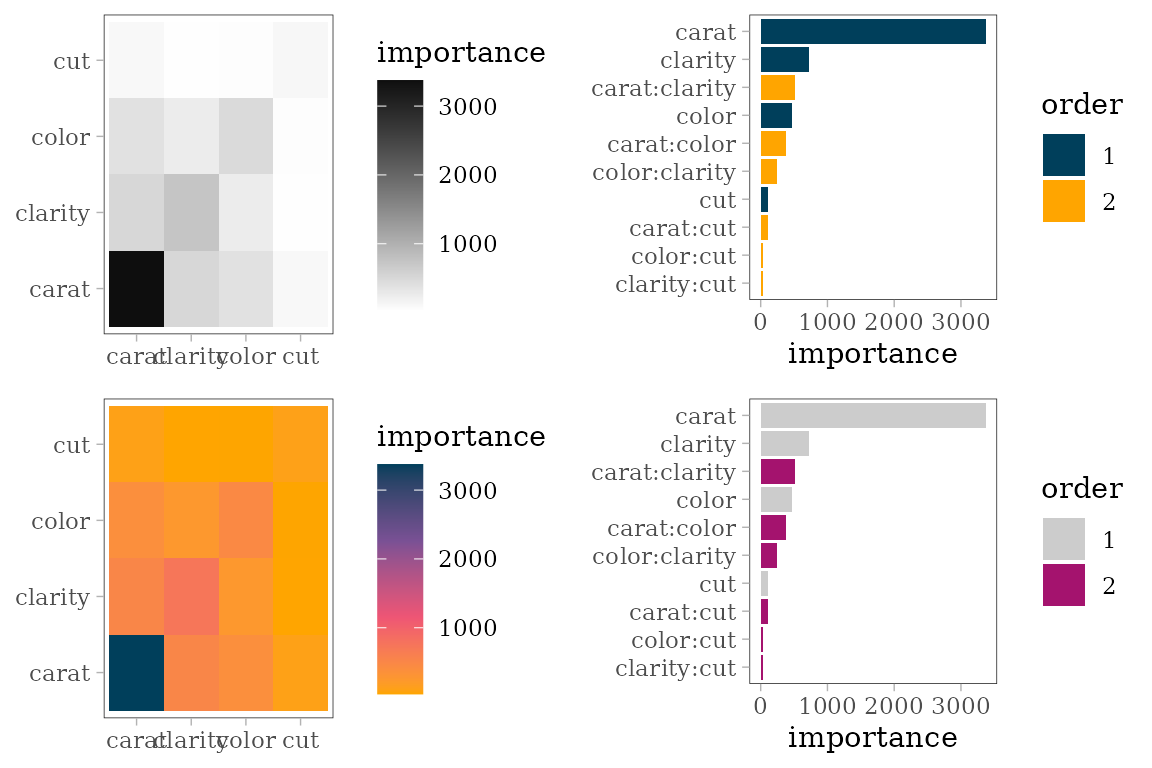
imp <- mid.importance(mid)
grid.arrange(
  ggmid(imp, "heatmap"),
  ggmid(imp, "barplot", max = 10, theme = "mytheme@q"),
  ggmid(imp, "heatmap", theme = "mytheme_r"),
  ggmid(imp, "barplot", max = 10, theme = "highlight_r")
)
Using themes with ggplot2
To apply your color themes to ggplot2 plots, use the
scale_color_theme() and scale_fill_theme()
functions. These scales integrate your themes directly into the plot’s
color and fill aesthetics.
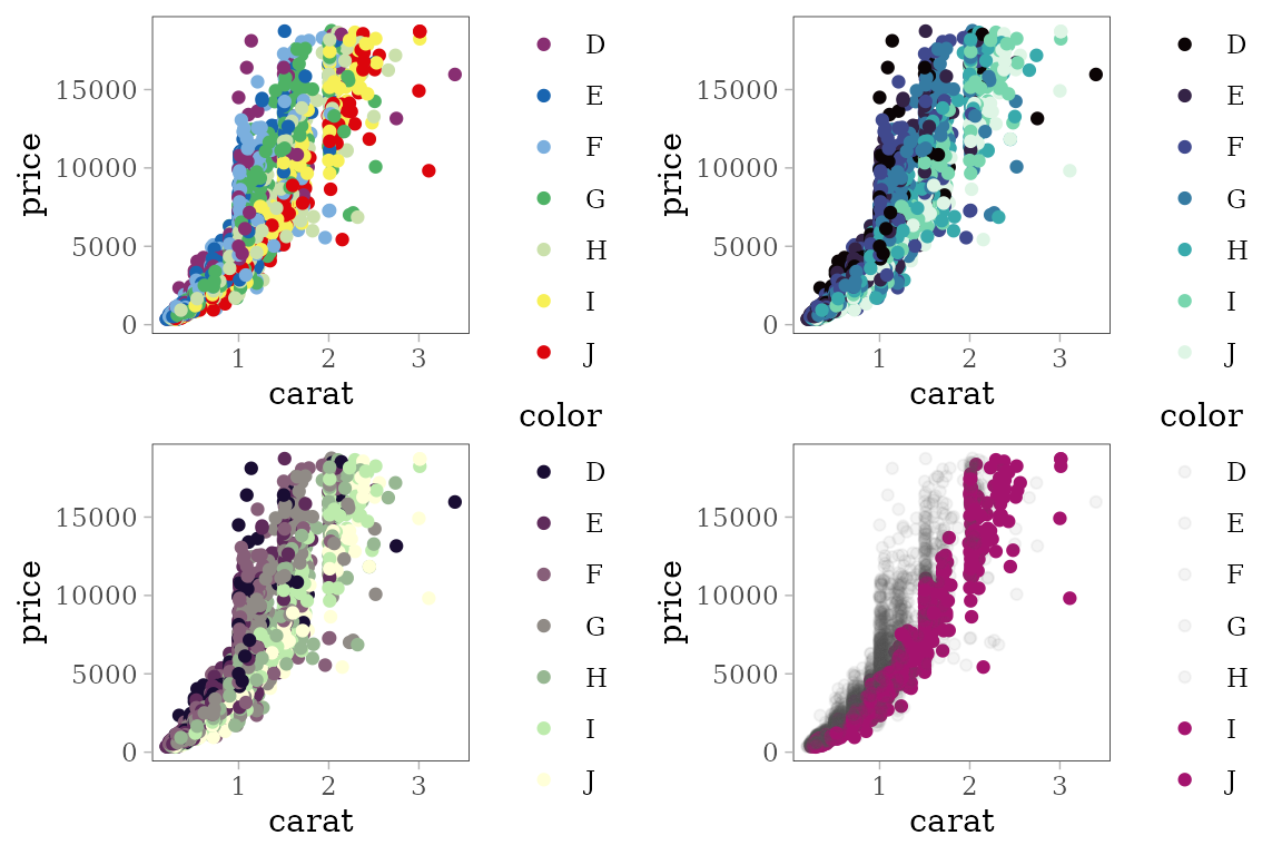
p <- ggplot(dataset) + geom_point(aes(carat, price, col = color))
grid.arrange(
  p + scale_color_theme("discreterainbow"),
  p + scale_color_theme("viridisLite/mako", discrete = TRUE),
  p + scale_color_theme("tokyo@qual"),
  p + scale_color_theme("highlight?base='#50505010'&which=6:7")
)
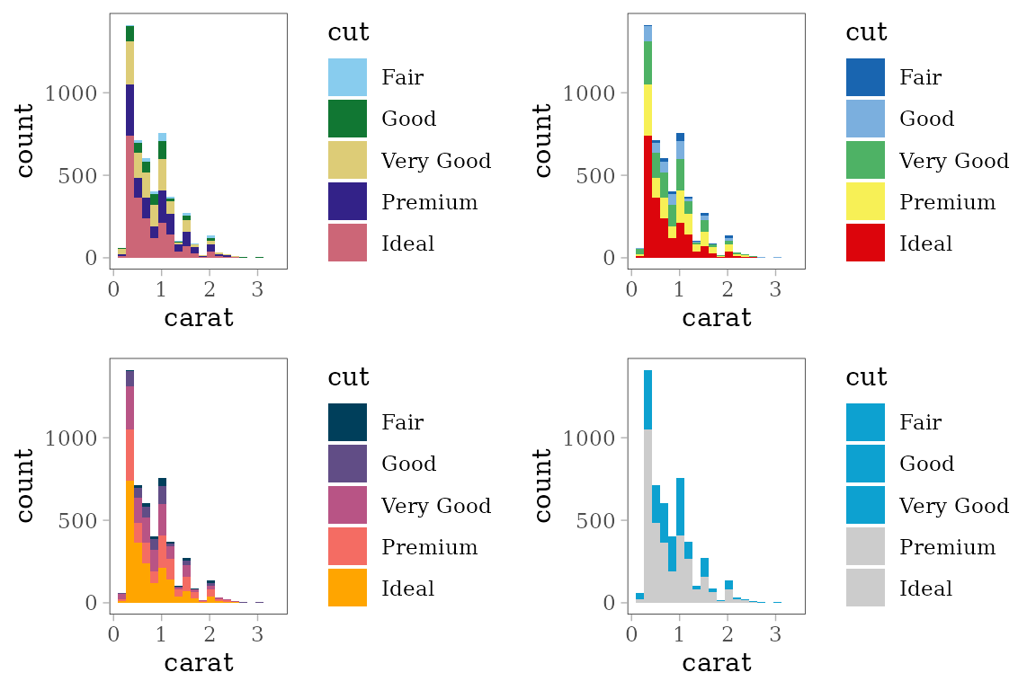
p <- ggplot(dataset) +
  geom_histogram(aes(x = carat, fill = cut), bins = 20)
grid.arrange(
  p + scale_fill_theme("muted_r"),
  p + scale_fill_theme("khroma/discreterainbow"),
  p + scale_fill_theme("mytheme@q"),
  p + scale_fill_theme("highlight?which=1:3&accent='#0da1d0'")
)