Interpretation of Classification Models • midr

This article presents some examples of the interpretation of classification models using midr.

# load required packages
library(midr)
library(ggplot2)
library(gridExtra)
library(Metrics)
theme_set(theme_midr())

Classification Task

We use the titanic dataset, which is available on the website https://www.encyclopedia-titanica.org/ and is included in the DALEX package. The dataset has 9 variables for 2207 people, of which 1317 were passengers and 890 were crew members. We fit some classification models that predict who survived the tragedy and who did not, and then we interpret the fitted models.

# benchmark classification task
library(DALEX)
#> Welcome to DALEX (version: 2.4.3).
#> Find examples and detailed introduction at: http://ema.drwhy.ai/
#> Additional features will be available after installation of: ggpubr.
#> Use 'install_dependencies()' to get all suggested dependencies
set.seed(42)
test_rows <- sample(nrow(titanic), 500L)
train <- titanic[-test_rows, -5]
str(train)
#> 'data.frame':    1707 obs. of  8 variables:
#>  $ gender  : Factor w/ 2 levels "female","male": 2 1 1 2 2 1 2 2 2 2 ...
#>  $ age     : num  42 39 16 25 30 28 27 20 30 27 ...
#>  $ class   : Factor w/ 7 levels "1st","2nd","3rd",..: 3 3 3 3 2 2 3 3 3 3 ...
#>  $ embarked: Factor w/ 4 levels "Belfast","Cherbourg",..: 4 4 4 4 2 2 2 4 4 4 ...
#>  $ fare    : num  7.11 20.05 7.13 7.13 24 ...
#>  $ sibsp   : num  0 1 0 0 1 1 0 0 0 0 ...
#>  $ parch   : num  0 1 0 0 0 0 0 0 0 0 ...
#>  $ survived: Factor w/ 2 levels "no","yes": 1 2 2 2 1 2 2 2 1 1 ...
test  <- titanic[ test_rows, -5]
str(test[, -9])
#> 'data.frame':    500 obs. of  8 variables:
#>  $ gender  : Factor w/ 2 levels "female","male": 2 2 1 2 2 2 2 2 1 2 ...
#>  $ age     : num  74 19 32 21 40 23 24 26 34 28 ...
#>  $ class   : Factor w/ 7 levels "1st","2nd","3rd",..: 3 3 2 3 4 3 5 5 2 5 ...
#>  $ embarked: Factor w/ 4 levels "Belfast","Cherbourg",..: 4 2 4 4 4 4 4 4 4 1 ...
#>  $ fare    : num  7.15 7.04 21 8.08 0 ...
#>  $ sibsp   : num  0 0 0 0 0 0 0 0 1 0 ...
#>  $ parch   : num  0 0 0 0 0 0 0 0 1 0 ...
#>  $ survived: Factor w/ 2 levels "no","yes": 1 1 2 1 1 1 2 1 2 2 ...

For each model type, we fit a classification model using the training dataset of 1707 people and an interpretative MID surrogate of the target model using the same dataset. We then evaluate the predictive accuracy of the target model by AUC and the representation accuracy of the surrogate model by the Spearman’s rank correlation coefficient between two predicted probabilities.

In the following examples, we use two specialized link functions for classification tasks: translogit (transformed-logit) and transprobit (transformed-probit). These two link functions are transformed so that $g(0.5) = 0.5$ and $g'(0.5) = 1$ . With these link functions, the effects on the linear predictor can be approximately interpreted as the upper bound of the effects on the predicted probabilities.

# define utility functions for the following chunks
effect_plots <- function(object) {
  plots <- mid.plots(mid, terms = terms(mid)[1:6])
  for (i in 1:6) {
    plots[[i]] <- plots[[i]] + ggtitle("main effect")
    if (any(i == c(1, 3, 4)))
      plots[[i]] <- plots[[i]] + coord_flip()
  }
  plots
}

interaction_plot <- function(
    object, term = NULL, theme = "shap") {
  if (is.null(term))
    term <- mid.terms(mid.importance(object), main.effect = FALSE)[1L]
  ggmid(object, term, type = "data", data = na.omit(titanic), 
        theme = theme, main.effects = TRUE) +
    theme(legend.position = "right") +
    ggtitle("interaction effect plot")
}

ice_plot <- function(object, variable = "age") {
  ggmid(mid.conditional(object, variable,
                        data = na.omit(titanic)[1:200, ]),
        var.color = gender, theme = "shap_r") +
    theme(legend.position = "right") +
    ggtitle("conditional expectation")
}

importance_plot <- function(object) {
  ggmid(mid.importance(object), "heatmap", theme = "grayscale") +
    theme(legend.position = "right") +
    ggtitle("feature importance")
}

evaluation_plot <- function(model, mid, ...) {
  pred <- get.yhat(model, test, ...)
  pred_mid <- get.yhat(mid, test)
  actual <- as.numeric(test$survived == "yes")
  auc_vs_test <- auc(actual, pred)
  cor_vs_mid <-  cor(pred, pred_mid, method = "spearman",
                     use = "pairwise.complete.obs")
  ggplot() + scale_color_theme("Accent") +
    geom_point(aes(x = pred, y = pred_mid), col = "#4378bf",
               data = na.omit(data.frame(pred, pred_mid))) +
    geom_abline(slope = 1, intercept = 0, col = "black", lty = 2) +
    theme(legend.position = "right") + xlim(0, 1) +
    labs(x = "model-prediction", y = "mid-prediction") +
    annotate("text", family = "serif", size = 3, x = 0.2, y = 0.8,
      label = sprintf("vs test (AUC)       : %.3f\nvs mid (Spearman): %.3f",
                      auc_vs_test, cor_vs_mid)
    ) + ggtitle("representation accuracy")
}

Additive Models

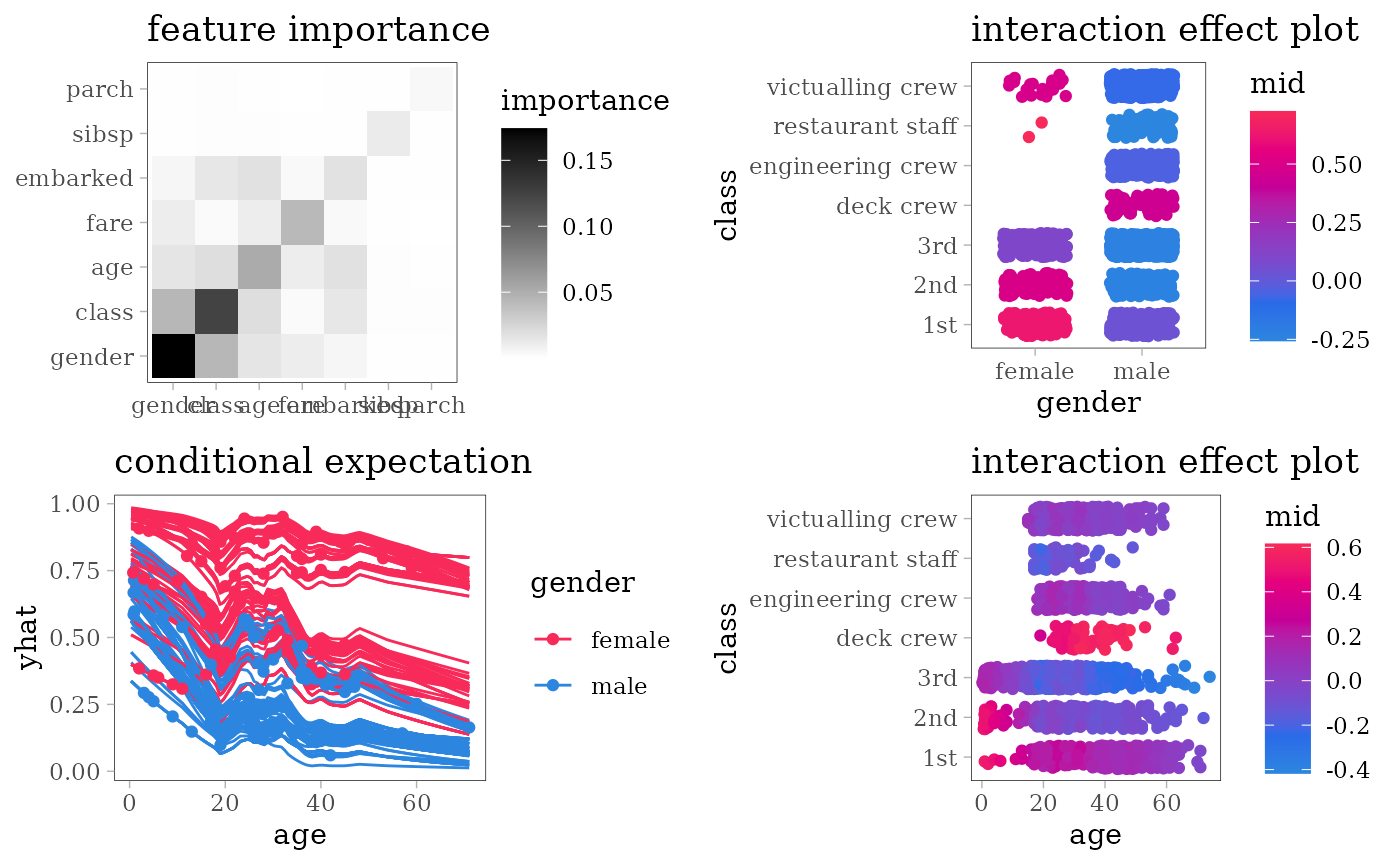
Logistic Regression

model <- glm(survived == "yes" ~ ., family = "binomial", data = train)
mid <- interpret(survived ~ .^2, train, model, link = "translogit")
print(mid)
#> 
#> Call:
#> interpret(formula = yhat ~ .^2, data = train, model = model,
#>  link = "translogit")
#> 
#> Model Class: glm, lm
#> 
#> Intercept: 0.26975
#> 
#> Main Effects:
#> 7 main effect terms
#> 
#> Interactions:
#> 21 interaction terms
#> 
#> Uninterpreted Variation Ratio: 0
grid.arrange(grobs = effect_plots(mid), nrow = 2L)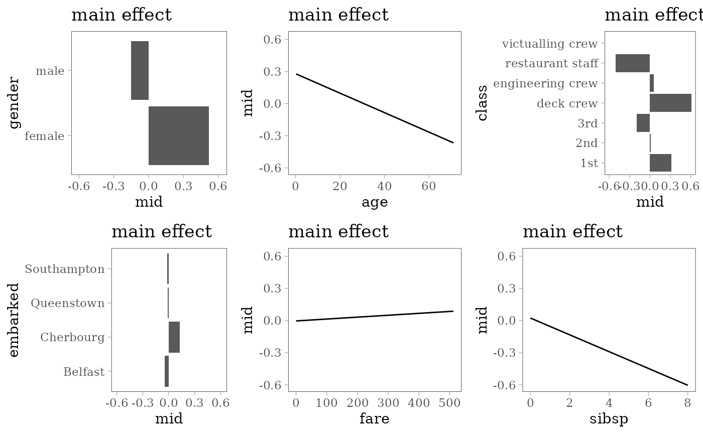

grid.arrange(nrow = 2L,
             importance_plot(mid),
             interaction_plot(mid),
             ice_plot(mid),
             evaluation_plot(model, mid, target = "yes"))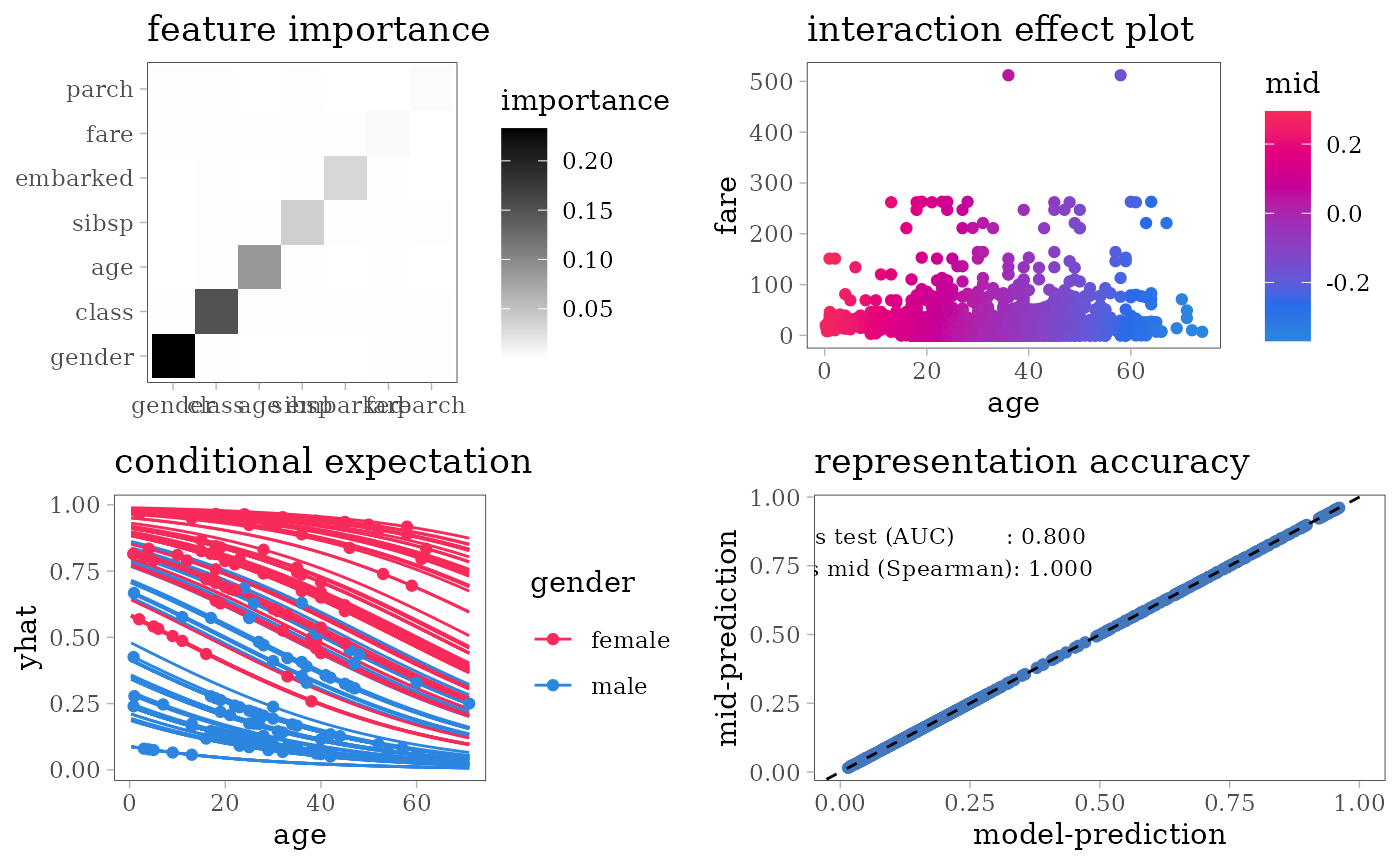

Neural Network

Single Hidden Layer Network

library(nnet)
set.seed(42)
model <- nnet(survived ~ ., train, size = 5, maxit = 1e3, trace = FALSE)
mid <- interpret(survived ~ .^2, train, model, link = "transprobit",
                 lambda = .01)
print(mid)
#> 
#> Call:
#> interpret(formula = yhat ~ .^2, data = train, model = model,
#>  link = "transprobit", lambda = 0.01)
#> 
#> Model Class: nnet.formula, nnet
#> 
#> Intercept: 0.29558
#> 
#> Main Effects:
#> 7 main effect terms
#> 
#> Interactions:
#> 21 interaction terms
#> 
#> Uninterpreted Variation Ratio: 0.045592
grid.arrange(grobs = effect_plots(mid), nrow = 2L)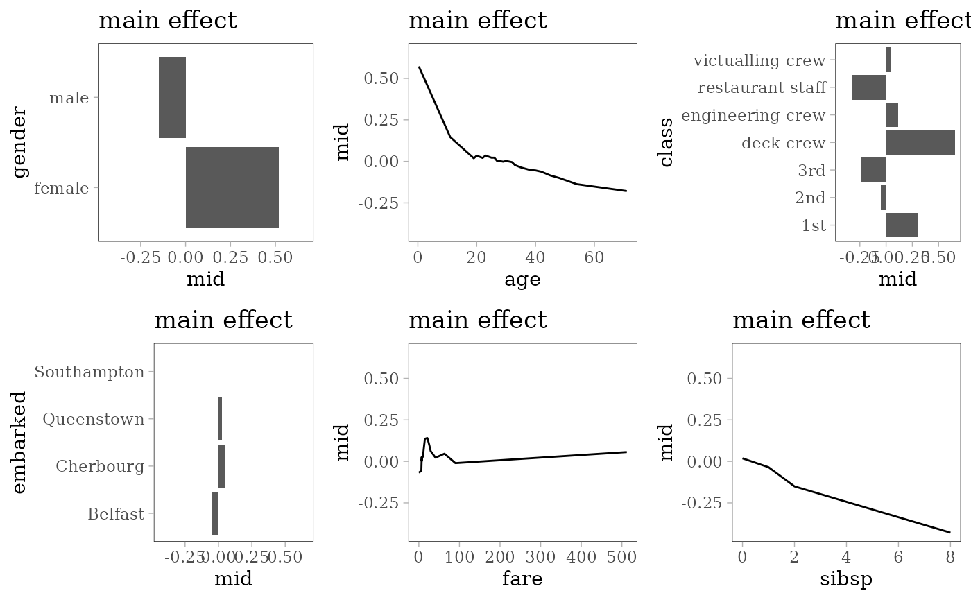

grid.arrange(nrow = 2L,
             importance_plot(mid),
             interaction_plot(mid),
             ice_plot(mid),
             evaluation_plot(model, mid))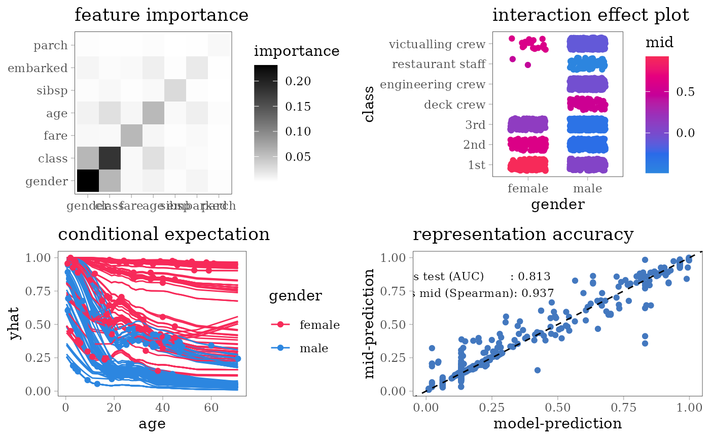

Support Vector Machine

RBF Kernel SVM

library(e1071)
model <- svm(survived ~ ., train, kernel = "radial", probability = TRUE)
mid <- interpret(survived ~ .^2, train, model, link = "transprobit",
                 pred.args = list(target = "yes"))
print(mid)
#> 
#> Call:
#> interpret(formula = yhat ~ .^2, data = train, model = model,
#>  pred.args = list(target = "yes"), link = "transprobit")
#> 
#> Model Class: svm.formula, svm
#> 
#> Intercept: 0.29569
#> 
#> Main Effects:
#> 7 main effect terms
#> 
#> Interactions:
#> 21 interaction terms
#> 
#> Uninterpreted Variation Ratio: 0.0073507
grid.arrange(grobs = effect_plots(mid), nrow = 2L)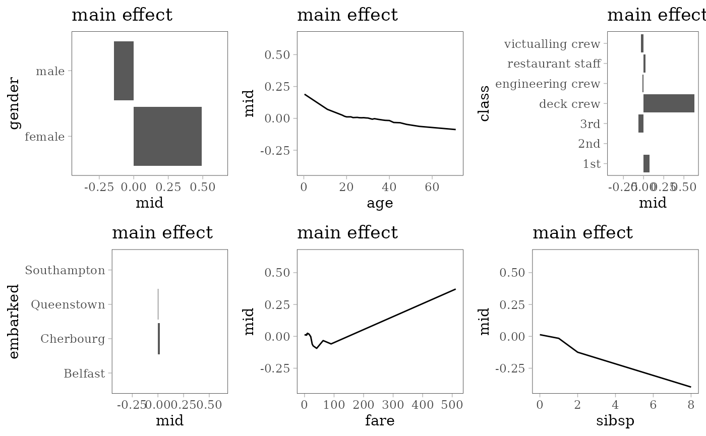

grid.arrange(nrow = 2L,
             importance_plot(mid),
             interaction_plot(mid),
             ice_plot(mid),
             evaluation_plot(model, mid, target = "yes"))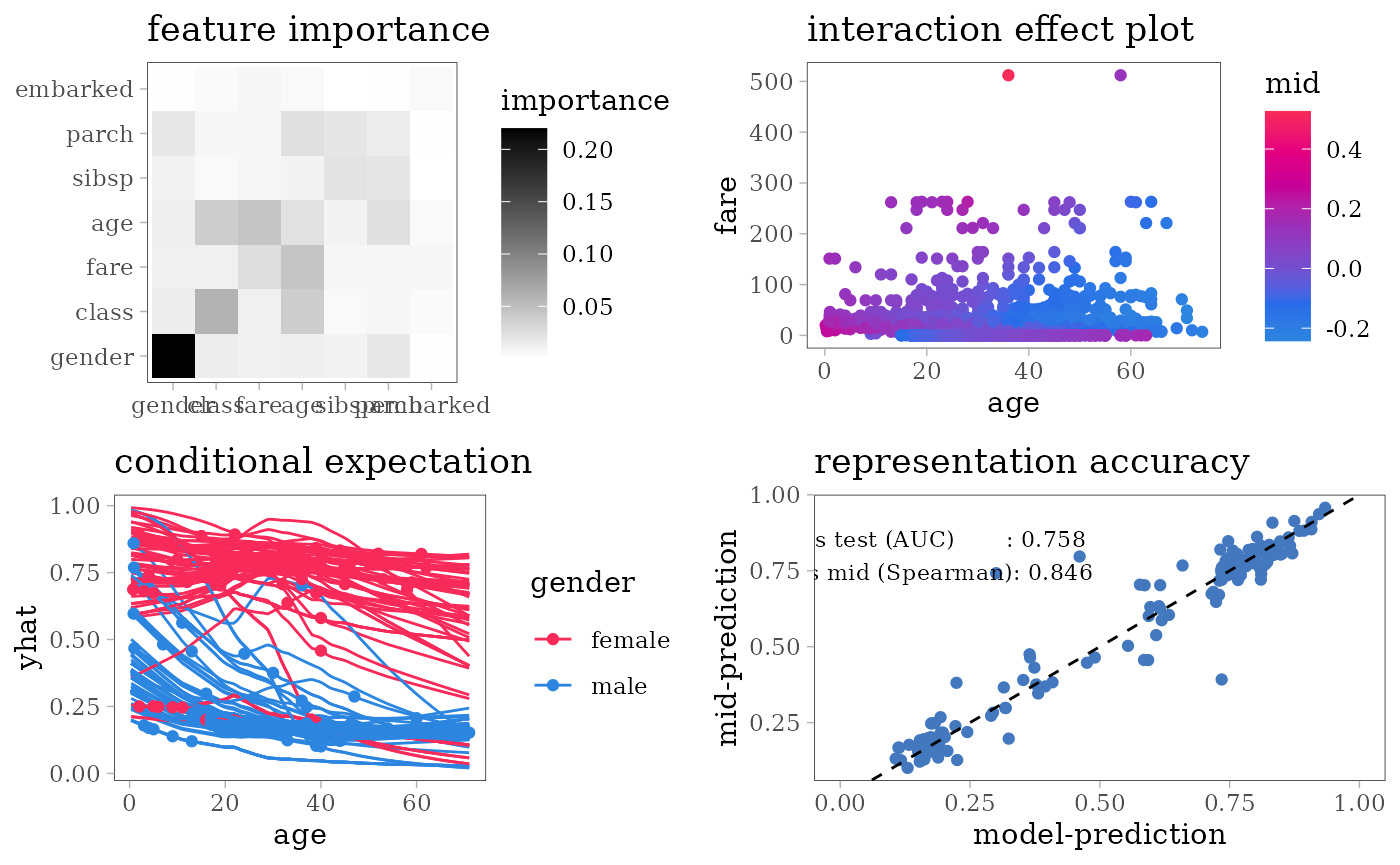

Tree Based Models

Random Forest

library(ranger)
set.seed(42)
model <- ranger(survived ~ ., na.omit(train), probability = TRUE)
mid <- interpret(survived ~ .^2, train, model,
                 link = "transprobit", lambda = .01)
print(mid)
#> 
#> Call:
#> interpret(formula = yhat ~ .^2, data = train, model = model,
#>  link = "transprobit", lambda = 0.01)
#> 
#> Model Class: ranger
#> 
#> Intercept: 0.30031
#> 
#> Main Effects:
#> 7 main effect terms
#> 
#> Interactions:
#> 21 interaction terms
#> 
#> Uninterpreted Variation Ratio: 0.062185
grid.arrange(grobs = effect_plots(mid), nrow = 2L)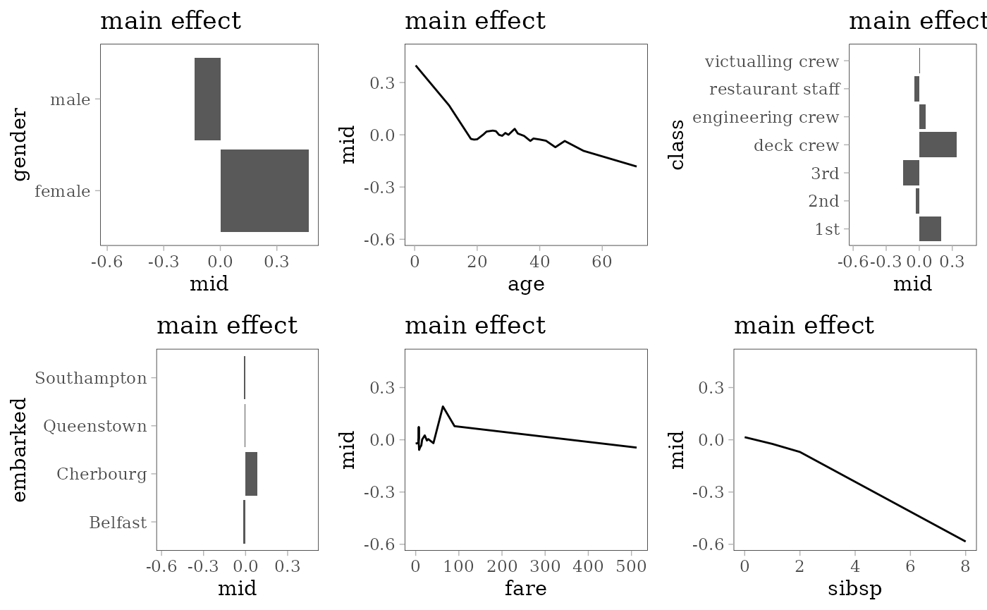

grid.arrange(nrow = 2L,
             importance_plot(mid),
             interaction_plot(mid),
             ice_plot(mid),
             evaluation_plot(model, mid, target = "yes"))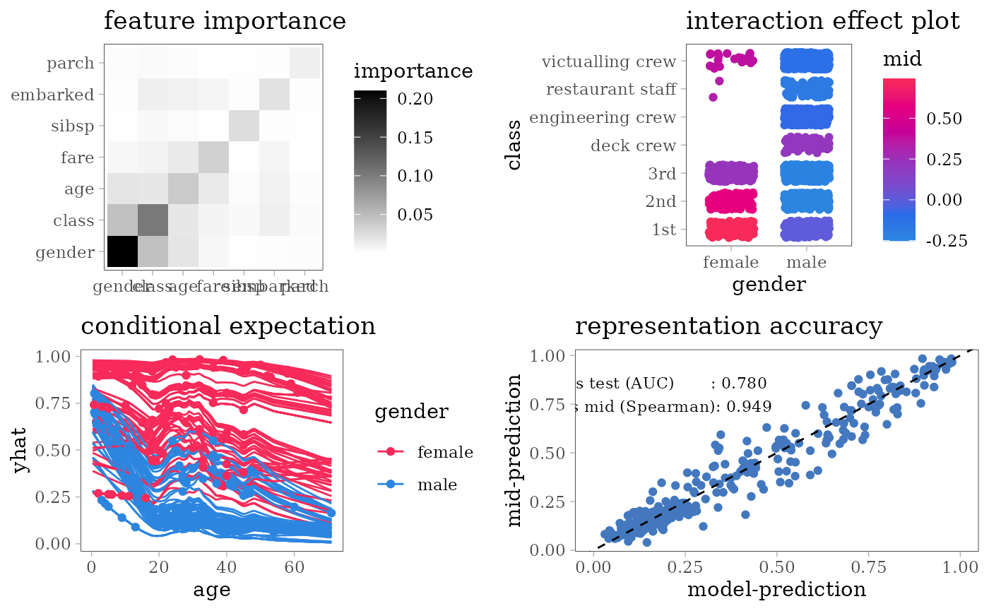

Decision Tree

library(rpart)
model <- rpart(survived ~ ., train)
# create encoding frames for CART
frm <- cbind(model$frame, labels(model, collapse = FALSE))
print(t(frm[frm$var != "<leaf>", c("var", "ltemp")]))
#>       1        2       4       9       5        11        3       6        
#> var   "gender" "class" "age"   "sibsp" "age"    "fare"    "class" "fare"   
#> ltemp "b"      "bcefg" ">=9.5" ">=2.5" ">=54.5" ">=26.63" "c"     ">=24.56"
#>       13      
#> var   "age"   
#> ltemp ">=36.5"
fun <- function(x) if (is.numeric(x)) range(x, na.rm = TRUE) else levels(x)
frames <- lapply(train, fun)
frames$age <- c(frames$age, 9.5, 54.5, 36.5)
frames$fare <- c(frames$fare, 26.63, 24.56)
frames$sibsp <- c(frames$fare, 2.5)
mid <- interpret(survived ~ .^2, train, model, link = "transprobit",
                 singular.ok = TRUE, type = 0, frames = frames)
#> singular fit encountered
print(mid)
#> 
#> Call:
#> interpret(formula = yhat ~ .^2, data = train, model = model,
#>  link = "transprobit", singular.ok = TRUE, type = 0, frames = frames)
#> 
#> Model Class: rpart
#> 
#> Intercept: 0.29099
#> 
#> Main Effects:
#> 7 main effect terms
#> 
#> Interactions:
#> 21 interaction terms
#> 
#> Uninterpreted Variation Ratio: 0.022918
grid.arrange(grobs = effect_plots(mid), nrow = 2L)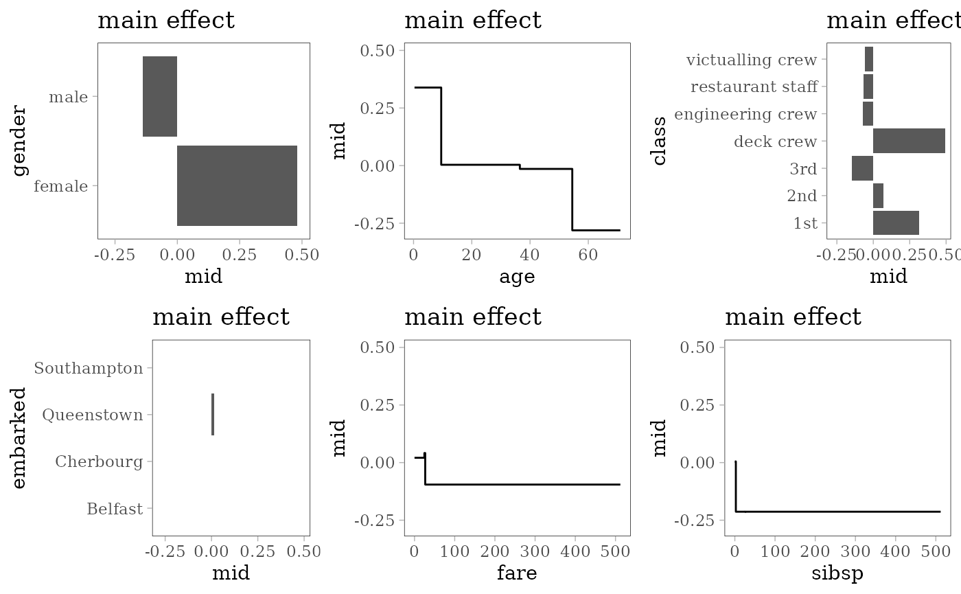

grid.arrange(nrow = 2L,
             importance_plot(mid),
             interaction_plot(mid),
             ice_plot(mid),
             evaluation_plot(model, mid, target = "yes"))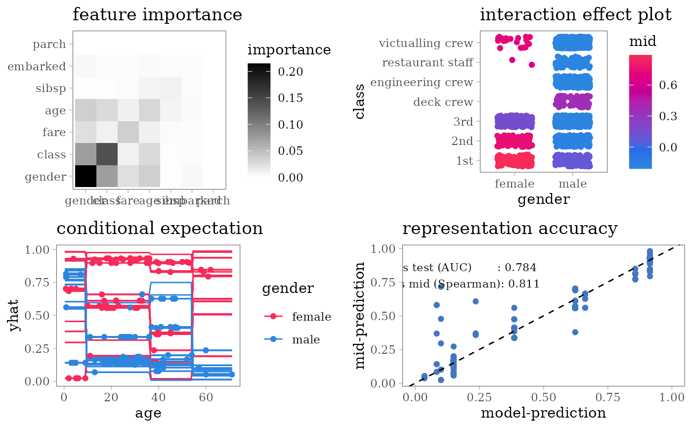

Other Models

Predictive MID

To fit a MID model for the Titanic classification task, we can use “one-sided” link functions: identity-gaussian or identity-logistic. These link functions map $0$ to $0$ and $1$ to $1$ , while the inverse link functions map any real number to the value in the unit interval $(0, 1)$ .

mid <- interpret(survived ~ .^2, train,
                 link = "identity-gaussian", lambda = .1)
#> 'model' not passed: response variable in 'data' is used
print(mid)
#> 
#> Call:
#> interpret(formula = survived ~ .^2, data = train, link = "identity-gaussian",
#>  lambda = 0.1)
#> 
#> Intercept: 0.32285
#> 
#> Main Effects:
#> 7 main effect terms
#> 
#> Interactions:
#> 21 interaction terms
#> 
#> Uninterpreted Variation Ratio: 0.61459
grid.arrange(grobs = effect_plots(mid), nrow = 2L)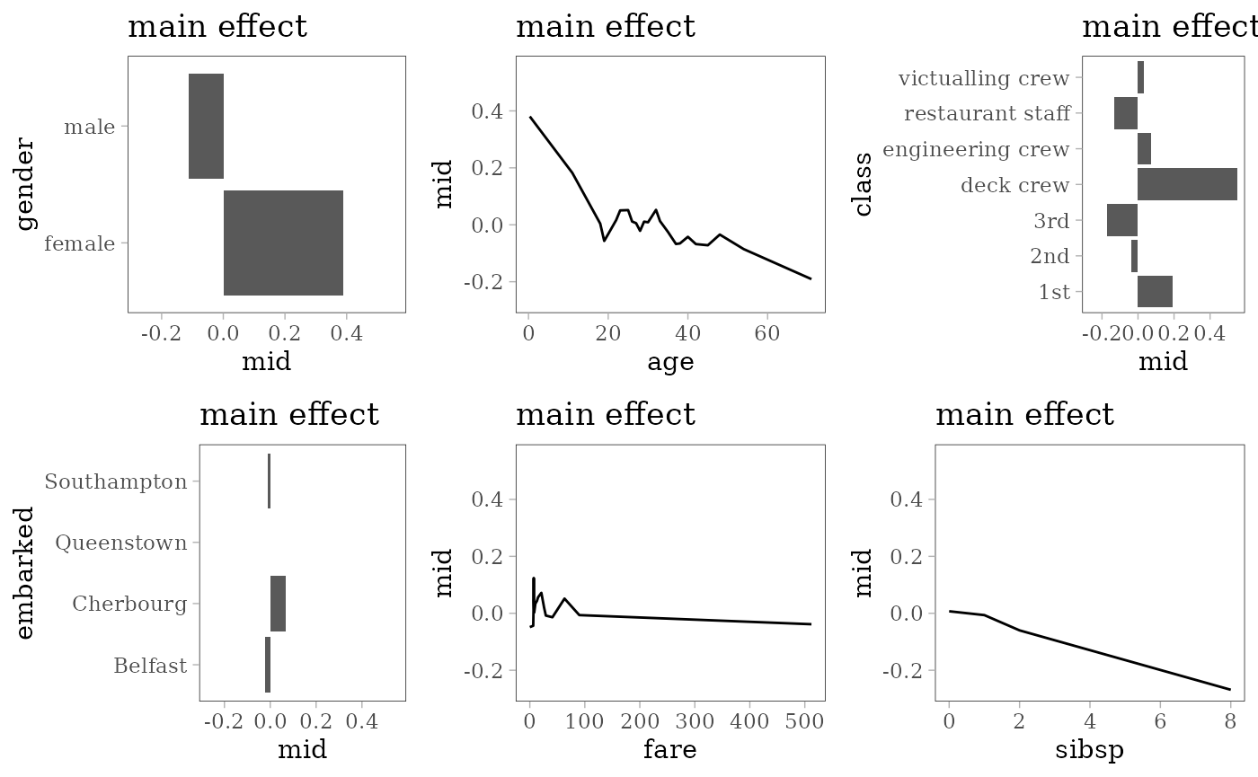

grid.arrange(nrow = 2L,
             importance_plot(mid),
             interaction_plot(mid),
             ice_plot(mid),
             interaction_plot(mid, "age:class"))