Getting Started with MID Collections

The midr package is designed not only to interpret individual models but also to facilitate comparative analysis. When you are dealing with multiple outcomes or comparing different modeling approaches, midr provides two specialized collection classes: “midlist” and “midrib”.

These collections allow you to visualize and compare feature effects, importance, and instance-level breakdowns across multiple models using a unified interface.

midlist: Flexible Combination of MID Objects

The “midlist” class is a versatile container used to group existing MID objects (such as mid, midimp, midbrk, or midcon). This is particularly useful when you have trained separate models—perhaps using different algorithms or targeting different subsets of data—and want to compare their behavior side-by-side.

Example: Comparing GAM vs. Random Forest

When predicting the total number of users (bikers) in the Bikeshare dataset, different machine learning algorithms capture non-linear relationships differently. Here, we fit a Generalized Additive Model (gam) and a Random Forest (ranger), interpret both of them independently, and unify the results into a single “midlist” collection for a direct visual comparison.

library(ggplot2)
library(patchwork)
library(midr)
library(gam)
library(ranger)

data(Bikeshare, package = "ISLR2")

fit.gam <- gam(
  bikers ~ mnth + hr + s(weekday) + weathersit + s(temp) + s(hum),
  data = Bikeshare
)

fit.ranger <- ranger(
  bikers ~ mnth + hr + weekday + weathersit + temp + hum,
  data = Bikeshare
)

# Interpret two separate models independently
mid.gam <- interpret(
  bikers ~ mnth + hr + weekday + weathersit + temp + hum,
  data = Bikeshare,
  model = fit.gam,
  k = 50
)

mid.ranger <- interpret(
  bikers ~ mnth + hr + weekday + weathersit + temp + hum,
  data = Bikeshare,
  model = fit.ranger,
  k = 50,
  lambda = 1
)

# Combine them into a midlist
mids <- midlist(
  gam = mid.gam,
  ranger = mid.ranger
)
class(mids)

#> [1] "mids"    "midlist"

When ggmid() is called on a “midlist” collection, it automatically handles the comparison.

options(midr.qualitative = "viridis")

p1 <- ggmid(mids, "hr") + theme(legend.position = "bottom")
p2 <- ggmid(mids, "temp") + theme(legend.position = "none")
p3 <- ggmid(mids, "hum") + theme(legend.position = "none")

p1 / (p2 + p3)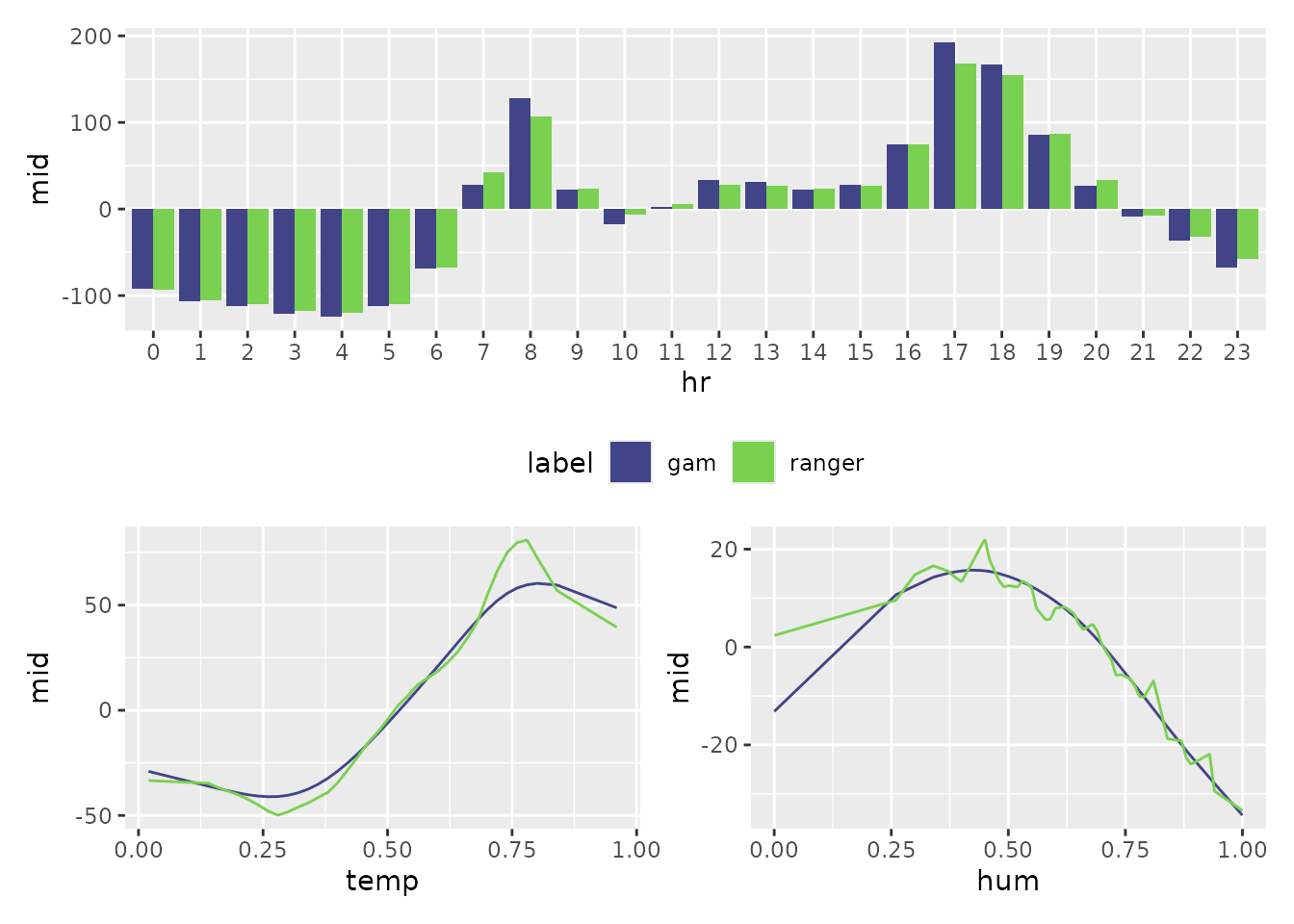

Mathematical Note: The “midlist” architecture offers maximum flexibility. Each model in the collection can maintain its own unique fitting parameters such as lambda (regularization strength), k (number of knots), and type (shape of component functions).

midrib: Efficient Multi-Response MID Model

The “midrib” class is designed for multi-output scenarios, where a single model predicts multiple target variables simultaneously. Instead of interpreting each response in isolation, midr treats the multi-output structure as a single entity—a “midrib” or shared backbone.

You can trigger the creation of a “midrib” object in two ways:

1. via formula: Provide a matrix or data frame as the response (e.g., using cbind()).
2. via prediction function: Pass a model and a custom pred.fun that returns a matrix or data frame of predictions.

Example: Joint Interpretation of Registered and Casual Users

Instead of comparing different algorithms, we might want to understand how features simultaneously affect different segments of our target variable. Here, we interpret a single model predicting both “registered” and “casual” users.

# Using a formula with a multi-column response
midrib <- interpret(
  cbind(registered, casual) ~ (mnth + hr + workingday + weathersit + temp + hum),
  data = Bikeshare,
  k = 50,
  lambda = 1
)

#> 'model' not passed: response variable in 'data' is used

class(midrib)

#> [1] "mids"   "midrib"

The resulting “midrib” object stores the fitted functions (i.e., all coefficients) for all outcomes in a unified structure, allowing for seamless comparative plotting.

options(midr.qualitative = "cividis")

p1 <- ggmid(midrib, "hr") + theme(legend.position = "bottom")
p2 <- ggmid(midrib, "temp") + theme(legend.position = "none")
p3 <- ggmid(midrib, "hum") + theme(legend.position = "none")

p1 / (p2 + p3)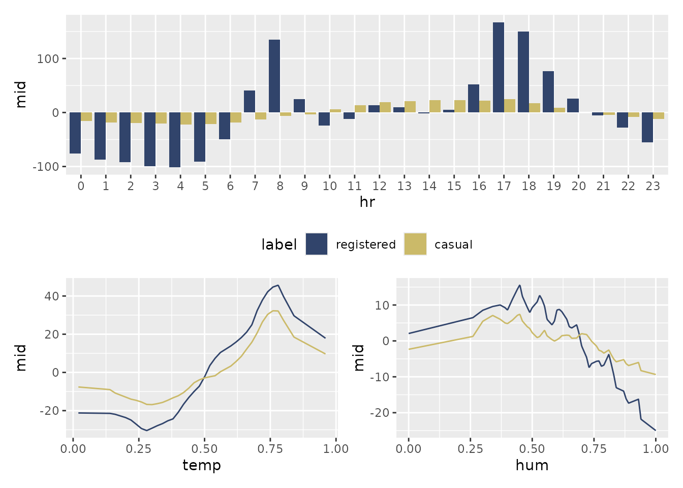

Mathematical Note: By sharing a single design matrix across all responses, the “midrib” class significantly reduces memory consumption and computation time. This makes it the ideal choice for high-dimensional multi-output data.

Summary of Collection Structures

Class	Data Structure	Optimization Logic	Key Advantage
“midlist”	A list of “mid”, “midimp”, “midbrk”, or “midcon”.	Independent: Each model has its own fitting parameters.	Flexibility: Compare heterogeneous models.
“midrib”	A single multivariate response model.	Joint: Shares a single design matrix across all responses.	Efficiency: Significant speedup for multivariate targets.