Compare MID Component Functions with ggplot2

For "mids" collection objects, ggmid() visualizes and compares a single main effect across multiple models.

Usage

# S3 method for class 'mids'
ggmid(
  object,
  term,
  type = c("effect", "series"),
  theme = NULL,
  intercept = FALSE,
  limits = c(NA, NA),
  resolution = NULL,
  labels = base::labels(object),
  ...
)

# S3 method for class 'mids'
autoplot(object, ...)

Arguments

object: a "mids" collection object to be visualized.
term: a character string specifying the main effect to evaluate.
type: the plotting style: "effect" plots the effect curve per model, while "series" plots the effect trend over models per feature value.
theme: a character string or object defining the color theme. See color.theme for details.
intercept: logical. If TRUE, the model intercept is added to the component effect.
limits: a numeric vector of length two specifying the limits of the plotting scale. NA values are replaced by the minimum and/or maximum MID values.
resolution: an integer specifying the number of evaluation points for continuous variables.
labels: an optional numeric or character vector to specify the model labels. Defaults to labels(object). The function attempts to parse these labels into numeric values where possible.
...: optional parameters passed to the main layer (e.g., linewidth, alpha).

Value

ggmid.mids() returns a "ggplot" object.

Details

This is an S3 method for the ggmid() generic that evaluates the specified term over a grid of values and compares the results across all models in the collection.

The type argument controls the visualization style. The default, type = "effect", plots the component functions of the specified term for each model individually. The type = "series" option transposes the view to plot the effect trend over the models for each feature value.

Note: Comparative plotting for interaction terms (2D surfaces) is not supported for collection objects.

Examples

# Use a lightweight dataset for fast execution
data(mtcars, package = "datasets")

# Fit two models with different complexities
fit1 <- lm(mpg ~ wt, data = mtcars)
mid1 <- interpret(mpg ~ wt, data = mtcars, model = fit1)
fit2 <- lm(mpg ~ wt + hp, data = mtcars)
mid2 <- interpret(mpg ~ wt + hp, data = mtcars, model = fit2)

# Combine them into a "midlist" collection (which inherits from "mids")
mids <- midlist("wt" = mid1, "wt + hp" = mid2)

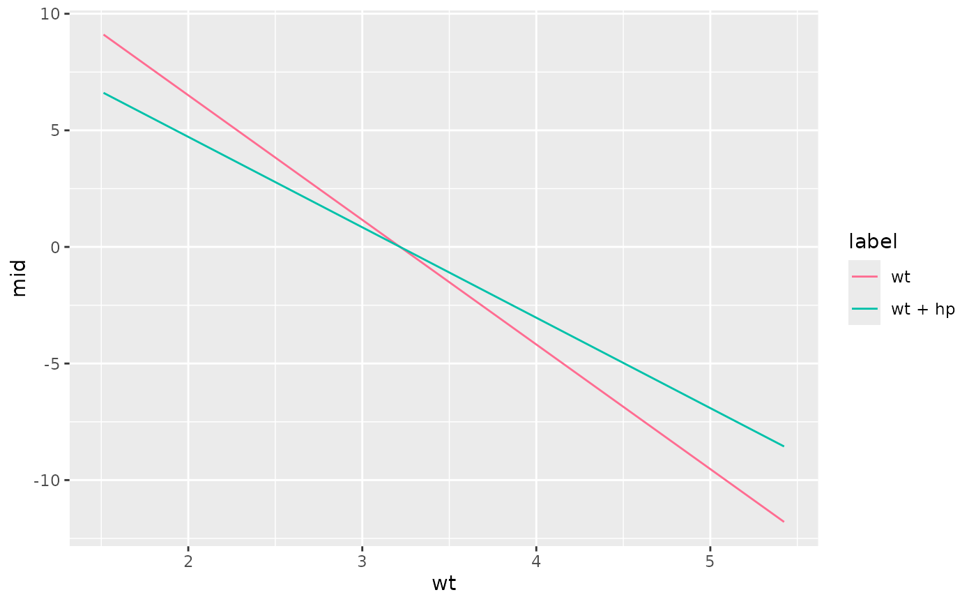
# Compare the main effect of 'wt' across both models
ggmid(mids, term = "wt")


# Compare the effect of 'wt' as a series plot across the models
ggmid(mids, term = "wt", type = "series")