Compare MID Conditional Expectations with ggplot2

For "midcons" collection objects, ggmid() visualizes and compares Individual Conditional Expectation (ICE) curves derived from multiple fitted MID models.

Usage

# S3 method for class 'midcons'
ggmid(
  object,
  type = c("iceplot", "centered", "series"),
  theme = NULL,
  var.alpha = NULL,
  var.linetype = NULL,
  var.linewidth = NULL,
  reference = 1L,
  sample = NULL,
  labels = NULL,
  ...
)

# S3 method for class 'midcons'
autoplot(object, ...)

Arguments

object: a "midcons" collection object to be visualized.
type: the plotting style. One of "iceplot", "centered", or "series".
theme: a character string or object defining the color theme. See color.theme for details.
var.alpha: a variable name or expression to map to the alpha aesthetic.
var.linetype: a variable name or expression to map to the linetype aesthetic.
var.linewidth: a variable name or expression to map to the linewidth aesthetic.
reference: an integer specifying the index of the evaluation point to use as the reference for centering the c-ICE plot.
sample: an optional vector specifying the names of observations to be plotted.
labels: an optional numeric or character vector to specify the model labels. Defaults to the labels found in the object.
...: optional parameters passed on to the main layer.

Value

ggmid.midcons() returns a "ggplot" object.

Details

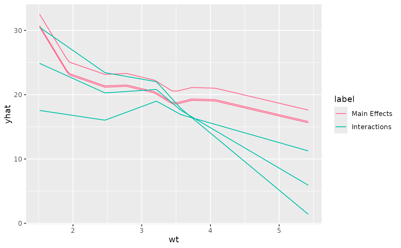
This is an S3 method for the ggmid() generic that produces comparative ICE curves from a "midcons" object. It plots one line for each observation in the data per model.

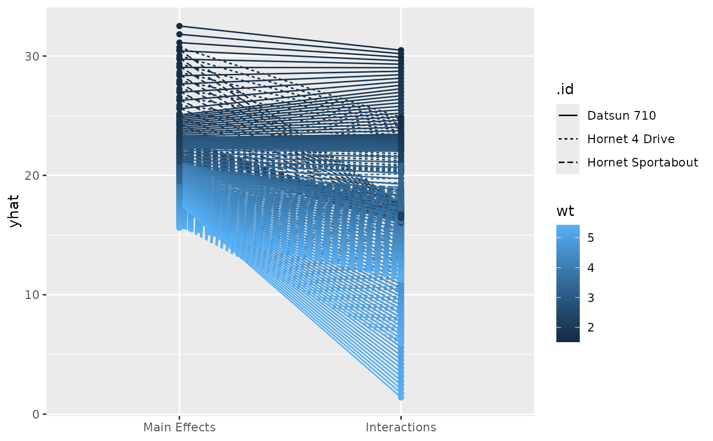
For type = "iceplot" and "centered", lines are colored by the model label. For type = "series", lines are colored by the feature value and plotted across models.

The var.alpha, var.linetype, and var.linewidth arguments allow you to map aesthetics to other variables in your data using (possibly) unquoted expressions.

Examples

data(mtcars, package = "datasets")

# Fit two different models for comparison
mid1 <- interpret(mpg ~ wt + hp + cyl, data = mtcars)
#> 'model' not passed: response variable in 'data' is used
mid2 <- interpret(mpg ~ (wt + hp + cyl)^2, data = mtcars)
#> 'model' not passed: response variable in 'data' is used

# Calculate conditional expectations for both models
cons <- midlist(
  "Main Effects" = mid.conditional(mid1, "wt", data = mtcars[3:5, ]),
  "Interactions" = mid.conditional(mid2, "wt", data = mtcars[3:5, ])
)

# Create an ICE plot (default)
ggmid(cons)


# Create a centered-ICE plot
ggmid(cons, type = "centered")


# Create a series plot to observe trends across models
ggmid(cons, type = "series", var.linetype = ".id")