library(lifecontingencies)lifecontingencies
パッケージの概要
lifecontingenciesは、ファイナンスや人口統計、保険数理の標準的な計算を実行することができるパッケージです。生命保険のリスク評価を実行するための包括的なツールセットとなっています。
データの取得
lifecontingenciesにはたくさんのデータセットが含まれています。以下にパッケージに含まれるデータセットの一覧を出力します。
# データセット一覧を取得
datasets_info <- as.data.frame(data(package="lifecontingencies")$results[,c("Item","Title")])
# 各データセットの型を取得し、一覧に追加
datasets_info$Class <- sapply(datasets_info$Item, function(x) class(get(x)))
# データセット一覧を出力
cat(apply(datasets_info, 1, function(x) paste(x, collapse = " : ")), sep = "\n")
AF92Lt : Uk AM AF 92 life tables : lifetable
AM92Lt : Uk AM AF 92 life tables : lifetable
SoAISTdata : SoA illustrative service table : data.frame
de_angelis_di_falco : Italian Health Insurance Data : list
demoCanada : Canada Mortality Rates for UP94 Series : data.frame
demoChina : China Mortality Rates for life table construction : data.frame
demoFrance : French population life tables : data.frame
demoGermany : German population life tables : data.frame
demoIta : Italian population life tables for males and females : data.frame
demoJapan : Japan Mortality Rates for life table construction : data.frame
demoUk : UK life tables : data.frame
demoUsa : United States Social Security life tables : data.frame
soa08 : Society of Actuaries Illustrative Life Table object. : lifetable
soa08Act : Society of Actuaries Illustrative Life Table with interest rate at 6 : actuarialtable
soaLt : Society of Actuaries life table : data.frame例えば、soaLtは古典的書籍『Actuarial Mathematics (Second Edition)』から参照された、年齢xと生存数I_xの2列から成るデータフレームです。
head(soaLt) x Ix
1 0 10000000
2 1 9949901
3 2 9899801
4 3 9849702
5 4 9799602
6 5 9749503tail(soaLt) x Ix
106 105 1668
107 106 727
108 107 292
109 108 108
110 109 36
111 110 11lifetable-class
lifetable型のオブジェクトは、年齢と各年齢に対応する生存数があれば作成でき、生存確率p_xと平均余命e_xを保持しています。
data.frame型であるsoaLtのデータセットから、with関数およびnew関数を利用してlifetable型のオブジェクトを作成し、このオブジェクトをもう一度data.frame型に変換し直すと、生存確率p_xと平均余命e_xの情報が追加されていることがわかります。
なお、lifecontingenciesにはsoa08というlifetable型のデータセットが含まれていますが、こちらは『Actuarial Mathematics (Second Edition)』のAppendix 2Aに掲載されているIllustrative life tableより作成されたもので、soaLtとは数値が異なります。
# soaLtの先頭行を出力。年齢xと生存数Ixの情報のみ。
head(soaLt)
x Ix
1 0 10000000
2 1 9949901
3 2 9899801
4 3 9849702
5 4 9799602
6 5 9749503# soaLtからlifetable型のオブジェクトsoaLt_lifetableを作成。
soaLt_lifetable <- with(soaLt, new("lifetable",x=x,lx=Ix,name="lifetable"))
str(soaLt_lifetable)Formal class 'lifetable' [package "lifecontingencies"] with 3 slots
..@ x : int [1:111] 0 1 2 3 4 5 6 7 8 9 ...
..@ lx : num [1:111] 10000000 9949901 9899801 9849702 9799602 ...
..@ name: chr "lifetable"# soaLt_lifetableをdata.frame型に変換(head関数を使用できるようにするため)。
soaLt_df <- as(soaLt_lifetable, "data.frame")
# 再び先頭行を出力。lifetable型のオブジェクトを作成したことで生存確率pxと平均余命exが取得できた。
head(soaLt_df) x lx px ex
1 0 10000000 0.9949901 71.34692
2 1 9949901 0.9949648 70.70616
3 2 9899801 0.9949394 70.06398
4 3 9849702 0.9949136 69.42035
5 4 9799602 0.9948876 68.77526
6 5 9749503 0.9990991 68.12867actuarialtable-class
actuarialtable型のオブジェクトは、年齢と各年齢に対応する生存数に加えて予定利率を設定すれば作成でき、計算基数を保持しています。
上述のlifetable型と同様の方法で、soaLtのデータセットからactuarialtable型のオブジェクトを作成し、計算基数の情報が追加されることを確認します。なお、ここでは予定利率を2.0%とします。
# soaLtの先頭行を出力。年齢xと生存数Ixの情報のみ。
head(soaLt)
x Ix
1 0 10000000
2 1 9949901
3 2 9899801
4 3 9849702
5 4 9799602
6 5 9749503# soaLtからactuarialtable型のオブジェクトsoaLt_actuarialtableを作成。
soaLt_actuarialtable <- with(soaLt, new("actuarialtable",interest=0.02,
x=x,lx=Ix,name="actuarialtable"))
str(soaLt_actuarialtable)Formal class 'actuarialtable' [package "lifecontingencies"] with 4 slots
..@ interest: num 0.02
..@ x : int [1:111] 0 1 2 3 4 5 6 7 8 9 ...
..@ lx : num [1:111] 10000000 9949901 9899801 9849702 9799602 ...
..@ name : chr "actuarialtable"# soaLt_actuarialtableをdata.frame型に変換(head関数を使用できるようにするため)。
soaLt_df2 <- as(soaLt_actuarialtable, "data.frame")
# 再び先頭行を出力。actuarialtable型のオブジェクトを作成したことで計算基数が取得できた。
head(soaLt_df2) x lx Dx Nx Cx Mx Rx
1 0 10000000 10000000 376393655 49117.059 2619732 161974034
2 1 9949901 9754805 366393655 48153.979 2570615 159354301
3 2 9899801 9515380 356638851 47209.784 2522461 156783686
4 3 9849702 9281594 347123471 46284.102 2475251 154261225
5 4 9799602 9053318 337841877 45376.570 2428967 151785974
6 5 9749503 8830425 328788559 7799.053 2383591 149357006生命年金の年金現価
lifecontingenciesに含まれているactuarialtable型のデータセットであるsoa08Actを用いて、様々な生命年金の年金現価を計算してみます。このデータセットはsoaLtと同じ生存数によるものですが、予定利率は6.0%です。なお、予定利率はaxn関数の引数にて新たに設定することも可能ですが、ここでは6.0%のままとします(以下に紹介する関数も同様)。
# 70歳開始の期始払終身年金の年金現価
axn(soa08Act, x=70, payment="advance")
[1] 8.569251# 60歳開始の期末払有期年金(10年)の年金現価
axn(soa08Act, x=60, n=10, payment="arrears")[1] 6.730136# 65歳開始(5年据置して70歳に初回支払)の期始払有期年金(15年)の年金現価
axn(soa08Act, x=65, n=15, m=5, payment="advance")[1] 5.164831また、x、n、mの引数はベクトルで設定することも可能です。
# 60~70歳開始の期始払終身年金の年金現価
axn(soa08Act, x=c(60:70), payment="advance")
[1] 11.145352 10.904118 10.658363 10.408367 10.154442 9.896928 9.636190
[8] 9.372622 9.106643 8.838698 8.569251# 60歳開始の期末払有期年金(5,10,15,20年)の年金現価
axn(soa08Act, x=60, n=c(5,10,15,20), payment="arrears")[1] 4.028154 6.730136 8.435766 9.414205生命保険の一時払保険料
同様に、soa08Actを用いて、様々な生命保険の一時払保険料を計算してみます。
# 30歳加入、保険期間10年の定期保険の一時払保険料
Axn(soa08Act, x=30, n=10)
[1] 0.01418541# 60歳開始、保険期間5年の養老保険の一時払保険料
AExn(soa08Act, x=60, n=5)[1] 0.7543062生命年金と同様に、引数はベクトルで設定することも可能です。
# 30歳加入、保険期間1~10年の定期保険の一時払保険料
Axn(soa08Act, x=30, n=c(1:10))
[1] 0.001442374 0.002872079 0.004292064 0.005705164 0.007114111 0.008521538
[7] 0.009929980 0.011341881 0.012759600 0.014185406生命保険の責任準備金
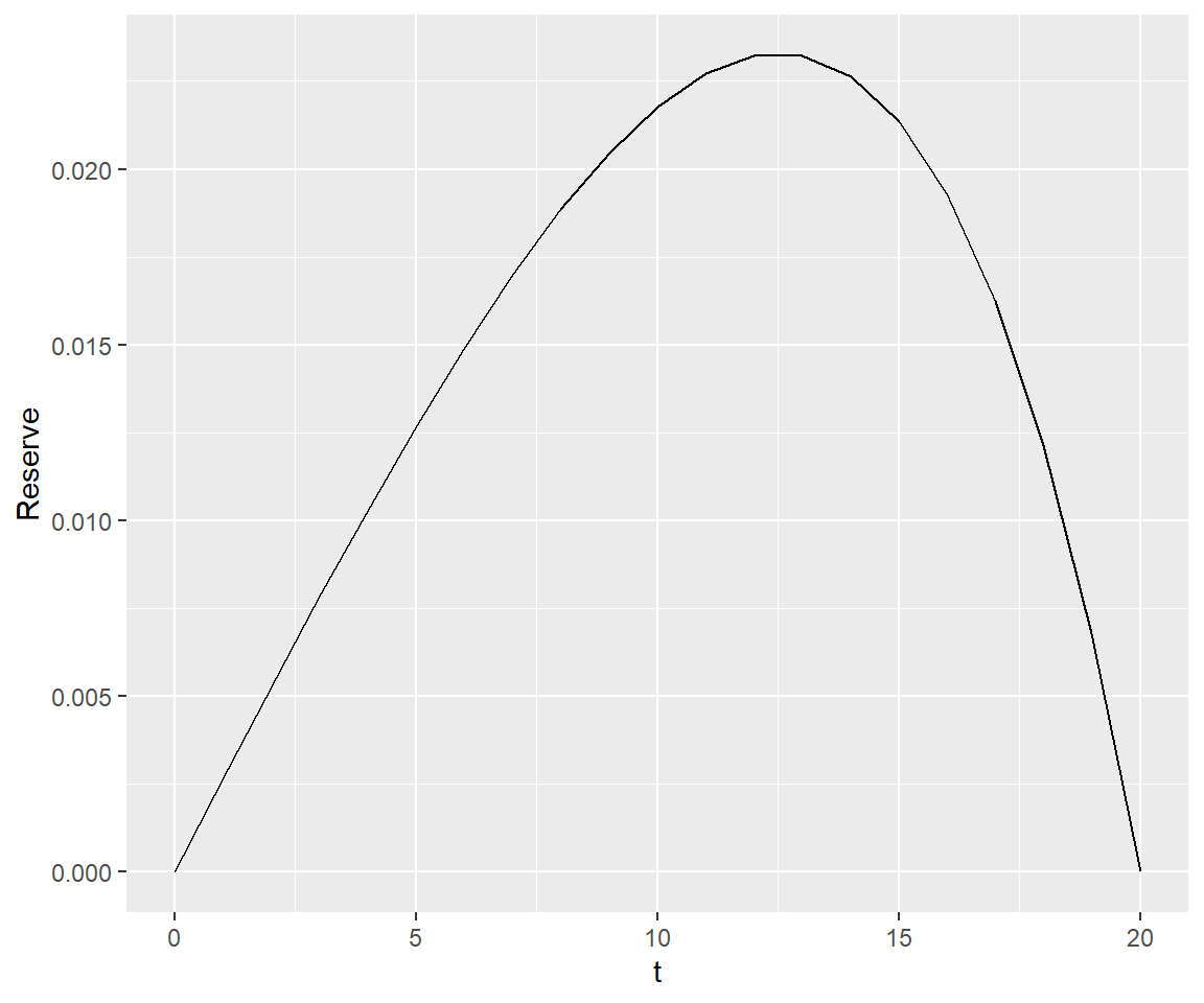
上記で紹介した関数を利用して、定期保険の純保険料式責任準備金を経過別に算出してみましょう。
# 40歳加入、保険期間20年の定期保険の年払純保険料
P <- Axn(soa08Act, x=40, n=20) / axn(soa08Act, x=40, n=20, payment="advance")
print(P)
[1] 0.005112706# 40歳加入、保険期間20年の定期保険の純保険料式責任準備金
V <- data.frame(t = numeric(21), Reserve = numeric(21))
for (t in 0:20){
V[t+1, 1] <- t
V[t+1, 2] <- Axn(soa08Act, x=40+t, n=20-t) - P * axn(soa08Act, x=40+t, n=20-t, payment="advance")
}
print(V) t Reserve
1 0 0.000000000
2 1 0.002645617
3 2 0.005257705
4 3 0.007815974
5 4 0.010297115
6 5 0.012674419
7 6 0.014917344
8 7 0.016991027
9 8 0.018855721
10 9 0.020466160
11 10 0.021770822
12 11 0.022711085
13 12 0.023220254
14 13 0.023222423
15 14 0.022631158
16 15 0.021347950
17 16 0.019260396
18 17 0.016240051
19 18 0.012139873
20 19 0.006791181
21 20 0.000000000# ggplotを使って責任準備金をプロット
library(ggplot2)
ggplot(V, aes(x = t, y = Reserve)) +
geom_line() +
labs(x = "t", y = "Reserve")